On Construction of Discontinuous Solutions for the Polynomial-like Iterative Equation
2018-11-06 03:20
长江大学学报(自科版) 2018年21期
[Abstract]Studying the solutions of the polynomial-like iterative equation is a significant subject in the research of dynamical systems because it closely relates to the data recovery and the invariant manifolds of systems.Much effort has been made to investigate its continuous and semicontinuous solutions, and many results are obtained.In this pa-per, firstly, we classify discontinuous self-maps into five subcases, and then with an extension method we give a general construction of discontinuous solutions of the polynomial-like iterative equation for each subcase.At last we apply main results to iterative roots.
[Keywords]polynomial-like iterative equation; discontinuous solutions; iterative roots
1 Introduction
The polynomial-like iterative equation:
α1f(x)+α2f2(x)+…+αnfn(x)=F(x)x∈I
(1)
is a linear combination of iterates of the unknown self-mapf:I→I,whereIis a closed interval ofR,F:I→Iis a given self-map andfi,i=2,3,…n,is thei-th iteration of the unknown self-mapf, i.e.,fi(x)=f(fi-1(x)) andf0(x)=x.In discrete dynamical system, data recovery is an important and interesting question.It results in theory of finding an n-order iterative root for a given functionF(see[1~3]).In other words, investigate the solutions offunctional equationfn(x)=F(x), which is a special form of (1).Invariant curve[2~5]is a part of research on invariant manifolds, which is an important problem in the study of dynamical systems because it can be used to reduce a system to a 1-dimensional one.While some problems related to invariant curves for planar mappings can be transformed into (1) withn=2 (see [6]).Hence equation(1) is one of important forms of functional equation.
For continuousF, existence and uniqueness of continuous solutions of equation (1) have been studied extensively ( see [7~15] ).Later, the results on smoothness and analyticity of solutions of equation (1) were investigated in [16~18].Convexity is one of the important properties of functions and often used in optimization, mathematical programming and game theory, so continuousconvex solutions of (1) also attracts great attentions ( see [19~21]).Recently, some attentions were paid for “complicated” functions such as multifunctions(see[22~25] ).
From the references above, we can see that these works mainly focus on the continuous and semicontinuous solutions of equation (1).However, most of practical dynamical systems possess the discontinuity, for instance, Poincaré map, doubling map and so on.One natural question is: whether equation (1) with discontinuous functionFpossesses discontinuous solutions under some conditions.This is an interesting and difficult object.The main difficulty comes from the discontinuous points (or called jumping points intuitively).In this paper, we deal with the discontinuous solutions of equation (1) with discontinuous functionF.Under the assumption thatαn≠0, one can divide equation (1)byαn, then equation (1) can be rewritten equivalently as:
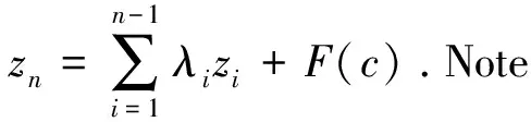
fn(x)=λn-1fn-1(x)+…+λ1f(x)+F(x)x∈I=[a,b]
(2)
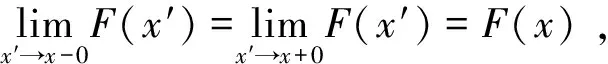
Whereλ1,λ2,…,λn-1are real constants andF:I→Iis a strictly increasing discontinuous function.Given a continuous pointξ∈IofF, as shown in [11], we also use the notationRξ,λ[I] for the classof strictlyincreasing
DiscontinuousfunctionsF:I→Isuch that:

(3)
(4)

(5)
(6)
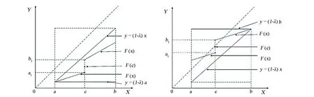
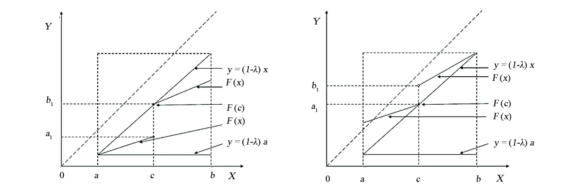
Figure 1 Ra,λ[I] Figure 2 Rb,λ[I]

Figure 3 Ra,λ[I1]∪F(c)∪Rb,λ[I2] Figure 4 Ra,λ[I1]∪F(c)∪Rb,λ[I2]

Figure 5 Ra,λ[I1]∪F(c)∪Rb,λ[I2]
2 Construction of Discontinuous Solutions
We will employ the following the lemma to construct discontinuous solutions of equation (2) with discontinuous functionF.This Lemma is similar to Lemma 2.1 presented in[11]so as to construct solutions of equation (2)with continuous functionF.
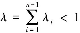
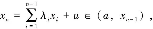
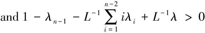
Lemma1Suppose that the coefficientsλiof equation (2), wherei=1,…,n-1, satisfy:
Then the following results hold:

ProofWe only prove (i), the other one can be proved similarly.Choose a positive constantLsuch that:
(7)
For an arbitrarily chosenx0∈(a,b], we can find a positive constantεsuch that:
(8)
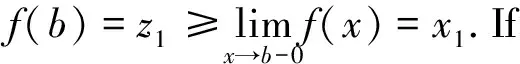
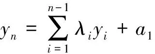
=xn-1 by(8).On the other hand, by (4) we obtain: The proof is completed. Using above lemma we can prove the following main theorems. Theorem1Under hypothesis (H), for a given discontinuous functionF∈Ra,λ[I],equation (2) has infinitely many discontinuous solutionsf∈Ra,0[I].Moreover, each of those solutions depends onn-1arbitrarilychosen orientation-preserving homeomorphismsfi:[xi,xi-1]→[xi+1,xi],i=1,2,…,n-1,wherex0,x1,…,xnare given as (i) in Lemma 1. Theorem2Under hypothesis (H), for a given discontinuous functionF∈Rb,λ[I],equation (2) has infinitely many discontinuous solutionsf∈Rb,0[I].Moreover, each of those solutions depends onn-1 arbitrarily chosen orientation-preserving homeomorphismsfi:[xi-1,xi]→[xi,xi+1],i=1,2,…,n-1,wherex0,x1,…,xnare given as (ii) in Lemma 1. We only prove Theorem 1 since Theorem 2 can be proved similarly. ProofofTheorem1Firstly, consider the case thatcis an endpoint ofI.cis the right endpoint ofIbecauseF∈Ra,λ[I].Letx0=c,by (ii) in Lemma 1, we can findn-1 pointsxi,i=1,2,…,n-1, such that: a (9) WhereNdenotes the set of all positive integers.Sincex0is a unique discontinuous point,Fis continuous on interval[a,x0).We assert that (xm) is a decreasing sequence in(a,x0]. In fact, it is trivial form=1,2,…,n.Suppose that this claim holds for all positive integersm≤k, wherek≥nis a certain integer.Thus we can get: (10) whereIm=[xm,xm-1].Next, it is ready to define mappingsfion those subintervals.For eachi=1,2,…,n-1,arbitrarily choose an orientation-preserving homeomorphismfi:Ii→Ii+1such that: fi(xi-1)=xifi(zi)=zi+1fi(xi)=xi+1 (11) zn∈[xn,xn-1) (12) =xn-1 Then, for eachm≥n, we recursively define: (13) We claim that for eachm∈Nmappingfm:Im→Im+1is an orientation-preserving homeomorphism and satisfies: fm(xm-1)=xm,fm(xm)=xm+1 =λn-1xk+λn-2xk-1+…+λ1xk-n+1+F(xk-n) =xk+1 Similarly, we can getfk+1(xk+1)=xk+2.Thus the claim is proved by induction. Finally, define: (14) Thenfis well defined on [a,b] andf∈Ra,0[I].Furthermore,forx∈(a,b) there existsm∈Nsuch thatx∈Im.Utilizing (13) and (14), we have: f(n)(x) =fn+m-1∘fn+m-2∘…∘fm+1∘fm(x)=λn-1fm+n-2∘…∘fm+1∘fm(x)+ λn-2fm+n-3∘…∘fm+1∘fm(x)+…+λ1fm(x)+F(x) =λn-1fn-1(x)+λn-2fn-2(x)+…+λ1f(x)+F(x) Which implies thatfdefined by (14) is a solution of equation (2) on[a,b).Sincef(b)=z1, from (11) we can get: fn(b)=fn-1∘f(b)=fn-1(z1)=fn-1∘fn-2∘fn-3∘…∘f2∘f1(z1)=zn On the other hand: λn-1fn-1(b)+λn-2fn-2(b)+…+λ1f(b)+F(b) =λn-1zn-1+λn-2zn-2+…+λ1z1+F(b) =zn Which implies: fn(b)=λn-1fn-1(b)+λn-2fn-2(b)+…+λ1f(b)+F(b) whereJm=[ym,ym+1].For eachi=1,2,…,n-1, arbitrarily choose an orientation-preserving homeomorphism. (15) (16) satisfies equation (2) onI.The proof is completed. By Theorem 1 and Theorem 2, we have the following corollary. Remark1The case thatb1=(1-λ)cshown in Fig.6 can be reduced to the subinterval [a,c), (c,b] and the single point set {c}.On the subintervals [a,c) and (c,b],we can obtain the solutions of equation (2) by Theorem 1 and 2, for the single point set {c}, we definef(c)=c.Thus we get infinitely many discontinuous solutions of equation (2).Similarly, for the casea1=(1-λ)cshown in Fig.7, we can obtain infinitely many discontinuous solutions of equation (2). Remark2One can apply our Theorem 1 and 2 to the case thatF∈Rξ,λ[I], wherea<ξ Figure 6 b1=(1-λ)c Figure 7 a1=(1-λ)c In the case thatn=2andλ1=λ2=0, equation (2) is transformed into the problem ofiterative roots for a given discontinuousF, i.e.: f2(x)=F(x) (17) Theorem3Suppose thatF:I:=[a,b]→Iis strictly increasing, discontinuous atc, wherec∈Iis the unique discontinuous point ofF.In addition,F(a)=a,F(b)=b(resp.ifcis an endpoint thenc=F(c)) andF(x) From Theorems 1, 2 and 3, we can obtain the following result: Corollary2Suppose thatF:I:=[a,b]→Iis strictly increasing, discontinuous at pointc,wherec∈Iis the unique discontinuous point ofF.In addition,F(a)=a,F(b)=b(resp.ifcis an endpoint thenc=F(c)) andF(x) fn(x)=F(x) has infinitely many discontinuous solutionsf∈Ra,0[I].

3 Application to Iterative Roots