A Computationally Hybrid Method for Solving a Famous Physical Problem on an Unbounded Domain

F.A.Parand,Z.Kalantari,M.Delkhosh,and F.Mirahmadian

1Department of Mathematics and Computer Science,Allameh Tabataba’i University,Tehran,Iran

2Department of Computer Sciences,Shahid Beheshti University,Tehran,Iran

3Department of Mathematics and Computer Science,Islamic Azad University,Bardaskan Branch,Bardaskan,Iran

Abstract In this paper,a hybrid method based on the collocation and Newton-Kantorovich methods is used for solving the nonlinear singular Thomas-Fermi equation.At first,by using the Newton-Kantorovich method,the nonlinear problem is converted to a sequence of linear differential equations,and then,the fractional order of rational Legendre functions are introduced and used for solving linear differential equations at each iteration based on the collocation method.Moreover,the boundary conditions of the problem by using Ritz method without domain truncation method are satisfied.In the end,the obtained results compare with other published in the literature to show the performance of the method,and the amounts of residual error are very small,which indicates the convergence of the method.

Key words:fractional order of rational Legendre functions,Newton-Kantorovich method,collocation method,Thomas-Fermi equation

1 Introduction

In the first of this section,an introduction of the spectral methods for solving the problems in the unbounded domains is presented.Then,the biography of Thomas-Fermi equation is investigated.

1.1 The Spectral Methods

Many of the problems in engineering sciences,astrophysics and other sciences occur in the unbounded domains.One of the best tools for solving these problems is the spectral methods.Spectral methods are one of the“big four” technologies for the numerical solution of ordinary differential equations(ODEs)which came into their own roughly in successive decades:(i)Finite Difference methods.[1−2](ii)Finite Element methods.[3](iii)Meshfree methods.[4−6](iv)Spectral methods.[7−9]The spectral methods have different approaches for solving the problems that defined in infinite and semi-infinite domains that presented in Table 1.

Table 1 Different approaches in spectral methods.

1.2 The Thomas-Fermi Equation

One of the most important nonlinear ordinary differential equations in atomic physics is the Thomas-Fermi equation.This problem that defined in unbounded domain is used for determining the effective nuclear charge in heavy atoms.The Thomas-Fermi equation is given as the following[25−26]

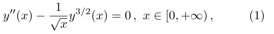
with the boundary conditions:

Importance of this problem in theoretical physics is caus-ing that computing its solutions have found many attentions in scientific research.

Also,the initial slope y′(0)of Thomas-Fermi equation plays an important role in determining many physical properties of this problem,therefore computing the value of y′(0)is very important in studies.

In recent years,different approaches are provided for solving Thomas-Fermi equation. Baker[27]has investigated singularity of this equation and has provided an analytical solution as follows:

where−A is the value of the first derivative at the origin.

Mason[28]has used rational approximations to the ordinary Thomas-Fermi functions and its derivative.Graef[29]has examined oscillatory and asymptotic properties of solutions of generalized Thomas-Fermi equations with deviating.MacLeod[30]has presented two differing approximations on Chebyshev polynomials,one for small x<40,and one for large x.

A numerical method on an unbounded interval for generation of enclosures based on monotone discretization principle and on available global bounds for the solutions of Thomas-Fermi equation have been investigated by Alzanaidi et al.[31]Development of a modification of the Adomian decomposition method that used several diagonal Pade approximates has studied by Wazwaz.[32]Also,during the years 2001 to 2011 different works for solving Thomas-Fermi problem have been presented,which some of them can be observed in Refs.[33–44].

In the year 2013,Boyd[45]has solved Thomas-Fermi equation.At the first,by using Newton-Kantorovich iteration method he reduced the nonlinear differential equation to a sequence of linear differential equations and then utilized a collocation method based on rational Chebyshev functions for solving this problem.The Sinc-collocation method for solving the Thomas-Fermi equation has provided by Parand et al.[46]The optimal Homotopy asymptotic method has used for solving the original Thomas-Fermi equation by Marinca et al.[47]Amor et al.[48]have studied the numerical integration,Power series with Pade,Hermite-Pade approximates,Pade-Hankel method and Chebyshev polynomials for solving Thomas-Fermi equation and obtained a highly solutions for this problem.The rational second-kind Chebyshev pseudospectral method has used for solving this problem by Kilicman et al.[49]Liu et al.[50]have presented an iterative method based on Laguerre pseudospectral approximation for solving Thomas-Fermi equation.In these studies,the solution of this problem is the sum of two parts include a power series expansion and a smooth part related to the singularity.Filobello et al.[51]have used the Thomas-Fermi equation as a case study for nonlinearities distribution Homotopy perturbation method.Combination of quasilinearization method and the fractional order of rational Chebyshev functions have presented by Parand et al.[52]Parand et al.[53]combined the quasilinearization method and the fractional order of rational Euler functions for solving Thomas-Fermi equation.Parand et al.[54]combined the quasilinearization method and the fractional order of rational Bessel functions for solving Thomas-Fermi equation.Parand et al.[55]combined the quasilinearization method and the fractional order of rational Jacobi functions for solving Thomas-Fermi equation.

2 Methodology

In this section,the work method has been investigated.

2.1 Fractional Order of Rational Legendre Functions

In this section,the Legendre polynomials and their basic properties are presented and then we have introduced the fractional order of rational Legendre functions on the unbounded domain.

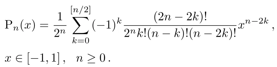
(i)Legendre Polynomials

These polynomials demonstrate as Pn(x).The Legendre polynomials have the expansion[56−57]

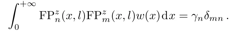
The distinct feature of the Legendre polynomials is that they are mutually orthogonal in the interval[−1,1]with respect to the uniform weight function w(x)=1,as follows:

where δmnis Kronecker delta.These polynomials satisfy the three-term recurrence relation:

The symmetric property for these polynomials is as follows:

Also,its derivative recurrence relation is:

(ii)The Fractional Order of Rational Legendre Functions

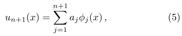
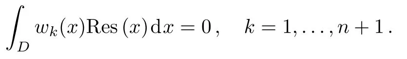
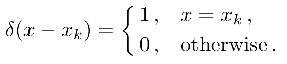
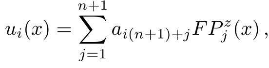
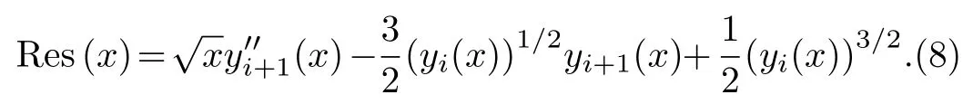
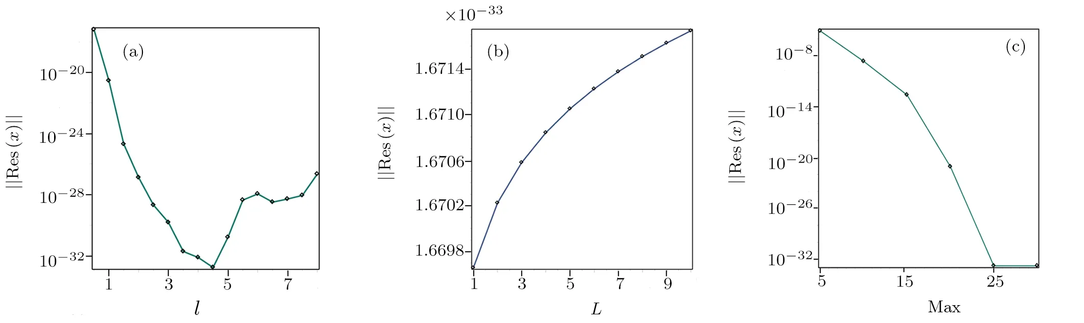
By using the change of variable(x−l)/(x+l),we can obtain rational Legendre polynomials,where l is a constant parameter and sets the length scale of the mapping.Boyd[58]has presented some techniques for finding the optimal value of l.Also,we define the fractional order of rational Legendre functions on the interval[0,+∞)by introducing the change of variable x→(xz−l)/(xz+l),l>0 and 0

Hence,we denote these functions by

and they obtain by using the following recurrence formula:

The derivative recurrence relation for these functions is as follows:

2.2 Newton-Kantorovich Method

The Newton-Kantorovich Method(NKM)represents an iterative approach combined with linear approximations.This method can be used to solve nonlinear problems in various sciences.In fact,the solution of nonlinear problems can be reduced to a sequence of linear problems by using this method.The advantage of the Newton-Kantorovich method for solving systems of nonlinear equations is its speed of convergence once a sufficiently accurate approximation is known.Some researchers have presented this technique in their lectures.[45,59−61]

Let L(m)(y(x))be one particular differential equation as follows:

where L(m)is the di ff erential operator of order m,andis a nonlinear function containing x,y(x),y(1)(x),y(2)(x),...,y(m−1)(x).The Newton-Kantorovich method yields the linear equations as follows:

where fy(j)is the derivate ofwith respect to y(j).

2.3 Collocation Method

One of the simple approaches to weighted residuals method is collocation method.[62]Therefore,we need to explain the method of weighted residuals at the first.Consider the initial-boundary-value problem of a differential equation

on a domain D for a function u(x)with boundary condition B(u)=0 and initial condition I(u)=0.To solving this equation,first make the approximate solution un+1(x)as a finite sum of known functions

where the ϕj(x)are called trial functions and ajare unknown coefficients.To solving Eq.(4),inserting the series expression(5)into Eq.(4)and define the residual function as follows:

To determine the n+1 unknown coefficients aj,the method of weighted residuals requires that the residual function Res(x)multiplied with n+1 test function wk(x)and integrated over the domain should vanish:

There exist various methods to choose the test functions.Here,we only mention the one most common approaches,namely the collocation method.In this method,a set of n+1 collocation points is chosen in the domain D on which the residual Res(x)is required to vanish

The consequence of this expression is that Eq.(4)is fulfilled exactly in the collocation points,L(un(x))|x=xk=0.Thus,the test functions become

with δ being the Dirac delta function

2.4 Solving Thomas-Fermi Equation

In this section,the explanation of our application for solving Thomas-Fermi equation is presented.In first,by using the Newton-Kantorovich method the nonlinear differential equation makes a sequence of linear differential equations.Afterward,the collocation method based on the fractional order of rational Legendre functions is applied for solving these linear equations.

So,by utilizing the NKM the answer of the Thomas-Fermi equation as the solution of the following linear differential equation in the(i+1)-th iterative approximation is determined by yi+1(x):

with the boundary conditions:

Due to the NKM-iteration needs initial guess of y0(x),its value prescribed y0(x)=1.Now,the collocation method is used to approximate the solution of the linear differential equation(6).

Therefore,we need to approximate the following function:

where ai(n+1)+jare unknown coefficient and n is the degree of the fractional order of rational Legendre function.Now,we consider:

where,the boundary conditions of Thomas-Fermi equation are satisfied and L is an arbitrary positive constant.Thus,at each iteration of the NKM,i=0,1,2,...,Max,the residual function is created by replacing yi+1(x)in the equation as follows:

Indeed,the residual function must be minimized in the any NKM-iteration.Therefore,by replacing the nodes xk,k=0,...,n which are the zeros of the fractional order of rational Legendre functions in the above equation,we obtain n+1 linear differential equations.Ultimately,the unknown coefficients can be found by solving these equations.Mandelzweig and Tabakin[33]have proved convergence of the NKM,and also Canuto et al.[63]and Guo[64]have proved the stability and convergence analysis of spectral methods,and,we will show that our numerical results are convergent.

3 Results and Discussion

As mentioned,Baker[27]has presented an analytical solution in the form Eq.(3)for Thomas-Fermi problem.The construction of this equation is based on the powers of x1/2,which actually this point is the cause of the choice of z=1/2 for solving this problem.

The numerical results for y(x)and y′(x)obtained by the present method with z=1/2,Max=25,l=4.5,L=1,and n=90 are displayed in Table 2.Also,we tabulate a list of potential y′(0)that calculated by researchers and the present method in Table 3.In this Table,accurate digits of y′(0)are in bold face.It can be observed that the obtained value y′(0)in the present method for n=90 is exact to 37 decimal places,which this point illustrates the convergence of the present method.

The approximate solution of y(x)by using the proposed method is depicted in Figs 1(a),and 1(b)presents the graphical demonstration of the absolute value of residual error.It is clear that amounts of residual error are very small,which this indicates the high accuracy of the present method.

Fig.1 (a)The graph of y(x). (b)The graphical demonstration of the absolute value of residual error with n=60,70,80,90 to illustrate the convergence of the method.

Figures 2(a)and 2(b)show the graphs ofof the present method at z=1/2,n=90 and the various values ofland L,respectively.The interval that we can choose for the parameters l and L to get applicable results are depicted in these figures.In particular,the reason why we select values l=4.5 and L=1 for solving this problem can be easily seen in these figures.

Also,Fig.2(c)indicates the graphs offor the various values of Max.It is seen that after the point Max=25,the changes in absolute errors ofare fixed.Therefore,in the present method Max=25 is the best value for solving this problem.

Table 2 Results of y(x)and y′(x)for the various values of x and n=90.

Table 3 Results of y′(0)in comparison with other researchers.

Fig.2 (a)The graphs of for the various l,(b)The graphs of for the various L,(c)The graphs of for the various Max,by the present method with z=1/2 and n=90.

4 Conclusions

The emphasis in this paper has been on solving nonlinear singular Thomas-Fermi equation.Our overriding aim has been to show that the combination of the Newton-Kantorovich and collocation methods can be applied easily to get high-accurate results for this problem.In order to evaluate the initial slope y′(0)that is very important in this problem,we obtain a good approximation y′(0)= −1.588 071 022 611 375 312 718 684 509 423 950 109 4 which is correct to 37 decimal places by using 90 collocation points,that is,we have obtained a more accurate solution by using fewer collocation points compared to other methods,other researchers have used 300 and 600 collocation points to obtain accuracy of 36 and 25 decimal places,respectively.Furthermore,a comparison between the obtained results of the present method and the results of variant methods that published in other lectures shows that proposed method is reliable and efficient.