
An Analysis of the Proton Structure Function and the Gluon Distributions at Small x
2019-01-10 06:58LuxmiMachahariandChoudhury
Luxmi Machahari and D.K.Choudhury
1Department of Physics,Gauhati University,Guwahati-781 014,India
2Physics Academy of North-East,Guwahati-781 014,India
Abstract Recently,we reported an analysis of Proton structure function at small x based on Taylor approximated DGLAP equations assuming a plausible relationship between the singlet and the gluon distributions.In this paper,we report a generalised version of the previous work.A corresponding study of the suggested gluon distribution is also made.The present generalised version of the model for the structure function results in a wider x range of phenomenological validity than the earlier one.A comparison of both the models of the proton structure function and the gluon distribution is made with exact result as well as with the Froissart saturated models of Block,Durand and Mckay.
Key words:small x,DGLAP equations,proton structure function,gluon distribution
1 Introduction
Study of the structure functions of proton and gluon distributions at small x is an active field of research since last several years.The standard tool to study small x physics is the DGLAP equations[1−4]to be followed by BFKL equations.[5−7]However in order to take into account the resummation of leading logarithmic terms and saturation effects thoroughly,more involved non-linear evolution equations like GLR,[8]Muller Qiu,[9]BK,[10−12]and JIMWLK[13−14]have emersed along with the notion of color glass condensate[15−16]since early 1980s with varying degrees of phenomenological success.[17−20]
Inspite of such advanced tools to study small x,DGLAP equations still survive at phenomenological level for its inherent simplicity.Approximate analytical forms of the proton structure function and the gluon distributions with plausible assumptions are too possible in such approach.
In this spirit,recently we reported an analysis[21]of the proton structure function(x,t)at small x based on Taylor approximated DGLAP equations assuming a plausible analytical relation[22]between the gluon G(x,t)and the singlet structure function(x,t)in conformity with observation of Lopez and Yndurain.[23]As Taylor approximated DGLAP equations are the first order differential equation in x and t,we solve them by the Lagrange’s Auxiliary method.[24]But the solution contains one undetermined parameter β.[25−26]For simplicity,the analysis of Ref.[21]has been reported setting it to be zero.The present work reports a generalised analysis without this assumption.In this paper,we will show that the positivity of the ratio of the parton distribution functions rules out a positive β while negative β has no such restrictions.Based on this observation,we will make a reanalysis of Ref.[21]and study if the phenomenological range of validity in x and Q2space reported earlier changes.The leading order structure function and gluon distribution is then compared with the exact results and also the corresponding models of the proton structure function and the gluon distribution suggested by Block,Durand and McKay.[27−28]
In Sec.2,we give a short outline of the formalism.Section 3 contains our result and the conclusions are highlighted in Sec.4.
2 Formalism
The standard coupled DGLAP equations for the singlet structure function and gluon distribution function at LO[29]are given respectively as
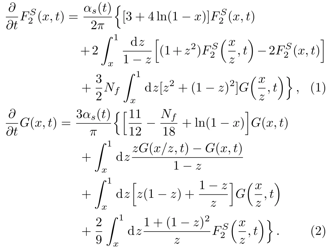
Here,αsis the strong coupling constant at LO given by αs(Q2)=12π/[(33− 2Nf)ln(Q2/Λ2)]and Λ is QCD scale parameter.Nfis the number of quark flavours,The other constants are TR=1/2,CA=3,CF=4/3.The singlet quark distribution is defined as

where qiandare quarks and antiquarks offl avour i.So singlet structure function is(x,t)=xΣ(x,t)and gluon distribution is G(x,t)=xg(x,t).

Equation(1)then becomes:[22]
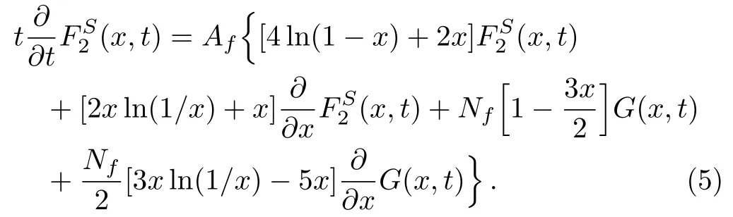
Similarly we obtain the Taylor approximated form of gluon DGLAP equation(2)as:

where Af=4/3β0and β0=(33 − 2Nf)/3.
Generally,the exact relation between the gluon distribution G(x,Q2)and the quark distribution

is not derivable in QCD even in leading order.However,if one assumes that at small x in a certain Q2range,such analytical form of the gluon and the quark distribution are possible,the most general form can be written as,
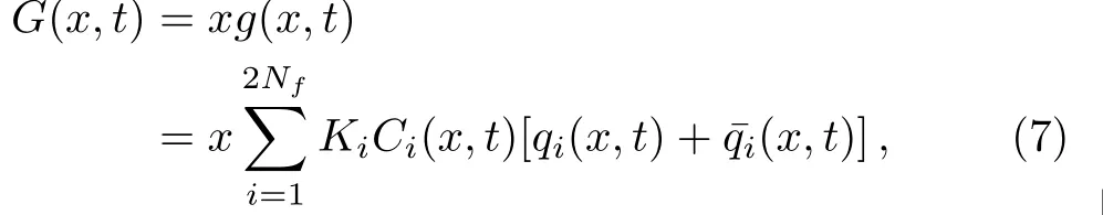
which takes into account the flavor independency of gluon.If the coefficients Kiand Ci(x,t)are also flavor independent then the expression can be written as

Here,KC(x,t)represent the ratio of the quark and gluon distribution and in general not factorizable in x and t.In Ref.[32],it was assumed that Q2dependence of both the distributions are identical while in Ref.[31],the following simple relation was assumed.

where k is a parameter to be determined from experiments.
A more rigorous analysis was done by Lopez and Yndurain[23]where they investigated the behaviour of the singlet structure function F2(x,Q2)and the gluon distribution G(x,Q2)at small x in leading order and obtained

where the functions BSand BGare Q2dependent.d+(1+λS)is the largest eigen value of the anomalous dimension matrix(Eq.(1.3b)of Ref.[23])and λSis strictly positive.From Eqs.(10)and(11)one infers that the ration between the gluon and the singlet structure function is only Q2dependent.That is,

The Q2dependence of KC(Q2)is not given by the current methods under study but is based on plausible physical reasons.The important characteristics of perturbative Quantum Chromo dynamics is the logQ2dependence as can be seen from the definition of the running coupling constant,as well as any Q2evolution of structure functions.A simple plausible theoretical form of KC(Q2)compatible with perturbative QCD expectation is[22]

where K and σ are two parameters to be fitted from experiments.Using Eq.(13),the above two Eqs.(5)and(6)become


The above two equations can be solved using the Lagrange’s Auxiliary method[24]and can be put in the following forms,

where,Q1(x,t),P1(x,t),R1(x,t),Q2(x,t),P2(x,t),R2(x,t)are explicit functions of K,t,σ as given in Appendix A.The solutions of Eqs.(16)and(17)are obtained by solving the following auxiliary system of ordinary differential equations,

Now if um(x,t)=Cmand vm(x,t,(x,t))=Dmare two independent solutions of the above Eqs.(16)and(17),then their general solutions can be written as[24]

where,fmare arbitrary functions of umand vm.
Solving the auxiliary equation(18),we get

where
To satisfy the general solution(19)the simplest possibility of finding a unique expression for(x,t)is the linear combination of umand vmin(x,t)such as,

where, α and β are two unknown quantities.Considering m=1,2 and putting the expressions for um(x,t)and vm(x,t,(x,t))in the above equation(28)we get the corresponding solution of Eq.(14)as

and solution of Eq.(15)as

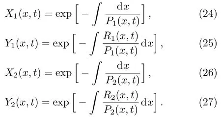
where the analytical expressions of X1(x,t),Y1(x,t),X2(x,t)and Y2(x,t)obtained in Ref.[21]are as given below:

From the analytical structures of X1(x,t),Y1(x,t),X2(x,t),and Y2(x,t)we observe that X1(x,t)̸=X2(x,t)and Y1(x,t)̸=Y2(x,t)and hence,the two evolutions defined in Eqs.(29)and(30)are not identical.We therefore de fine them asandrespectively.
However at certain t=t0,we use the boundary condition

It will result in two alternative inequivalent forms of t evolution for singlet distribution as

With ratio

which is not unity in general.
From Eqs.(31),(32),(33),and (34)weobserve that the ratio X1(x,t)/X1(x,t0),Y1(x,t0)/Y1(x,t),X2(x,t)/X2(x,t0),and Y2(x,t0)/Y2(x,t)as occured in Eq.(38)are invariably positive.Therefore for a negative β,R(x,t)will be positive de finite.However for a certain positive value of β(>0),positivity of the ratio R(x,t)defined in Eq.(38)is not assured in a certain speci fic range of x and t where,


Numerical analysis with positive and negative β will be reported in the following section.
3 Results
3.1 Analysis of the Parton Distribution Functions with Non-Zero β
(i)Analysis with positive β

Fig.1 for β positive.

Fig.2 for β positive.
(ii)Analysis with negative β
When β is negative both the structure functionsandwill be positive(>0)for the representative values of x and Q2(2×10−7,4 GeV2),(2×10−2,4 GeV2),(3×10−6,400 GeV2)and(3×10−2,400 GeV2)respectively as shown in Figs.3 and 4.

Fig.3 or β negative.

Fig.4 for β negative.
Using the same values of K and σ as in Ref.[21],we fit both Eqs.(36)and(37)with available globally obtained PDFs like NNPDF3.0[33]data in Mathematica and obtain the best fitted values of β for both the equations respectively.
We have used the HERAPDF1.0[34]input for evolution of our solutions with Q2=1.9 GeV2.For(x,t)of the 1stevolution Eq.(36),we obtain the best fitted value of β to be −2.69 at x=2 × 10⁻³and fixed range of Q:1.4 GeV≤Q≤100 GeV.

Fig.5 with fitted β = −2.69,K=2.7225 and σ =0.7112 and with fitted β = −0.364,K=2.7225,and σ=0.7112,and comparison with the data.[33,35]

Fig.6 with fitted β = −1.016,K=1.856 and σ =0.227 and with fitted β = −13.126,K=0.89 and σ=1.594,and comparison with the data.[33,35]
Let us also discuss our another choice of negative β where,positive K and σ are made to vary without prior inputs on K and σ.We obtain the best fitted value of β,K and σ forto be-1.016,1.856 and 0.227 respectively(third row of Table 1)and forto be-13.126(putting the constraint of β<0 during the fit in Mathematica),0.89 and 1.594 respectively(third row of Table 1)and forto be −13.126(putting the constraint of β <0 during the fit in Mathematica),0.89 and 1.594 respectively(third row of Table 2).
Table 1 Phen omenological paramters and the range of validity in x offor fixed Q range:2 GeV≤Q≤100 GeV.

Table 1 Phen omenological paramters and the range of validity in x offor fixed Q range:2 GeV≤Q≤100 GeV.
FS(I)2 (x,t)βK σ x range 0 2.7225 0.7112 2.10−6≤ x≤ 5.10−4–2.69 2.7225 0.7112 5.10−4≤ x ≤ 2.10−3–1.016 1.856 0.227 2.10−6≤ x ≤ 1.10−3
Table 2 Pheno menological parameters and the range of validity in x offor fixed Q range:2 GeV≤Q≤100 GeV.

Table 2 Pheno menological parameters and the range of validity in x offor fixed Q range:2 GeV≤Q≤100 GeV.
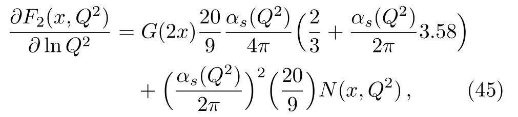
FS(II)2 (x,t)β K σx range 0 2.7225 0.7112 2.10−3≤ x≤ 5.10−3–0.364 2.7225 0.7112 1.10−3≤ x ≤ 2.10−3–13.126 0.89 1.594 0.01 We thus obtain their corresponding singlet structure functionsusing their proper choices of negative β,positive K and σ values.In Fig.5 we plot the two model structure functions evolving with Q for a few representative values of x and then compare with the recent available PDF data sets.[33,35] Observations from Figs.5 and 6 of the phenomenological range of validity in x for Q range 2 GeV≤Q≤100 GeV forandare recorded in Tables 1 and 2 respectively. In our previous work,[21]we obtainedmore favoured thanwith its phenomenological x range of validity forto be within 2×10⁻⁶≤ x≤5×10⁻⁴and 2 GeV ≤ Q≤ 100 GeV.In this present work too the preference ofis seen overon a proper choice of negative β and positive K and σ.From Tables 1 and 2,it is observed thatwith β = −1.016,K=1.856,and σ =0.227 is the most favoured among all the three sets of choices with its increasing phenomenological x range 2×10⁻⁶≤ x ≤ 1×10⁻³with same Q range.So generalisation of our previous model[21]to β ̸=0 gives a wider range of small x for a proper choice of β,K,and σ. (iii)Comparison with the phenomenological model of Block Durand et al The Froissart saturated phenomenolgical model of structure function and the gluon distributions proposed by Refs.[27–28]have attracted considerable amount of interest in recent literature.We therefore compare the present model ofwith this model where the exact analytical struction ofis as given below: where, Fig.7 Comparison of (x,t)using β = −1.016,K=1.856,σ =0.227 with the model of Block et al.[27] a0,a1,a2,b0,b1,b2are as given in Appendix B.In Fig.7 we plot the most favouredusing β = −1.016,K=1.856,σ =0.227 within our range of validity at three representative values of x(x=8×10−5,5×10−4,1×10⁻³)and then compare it with the phenomenologically model of Block,Durand and Mckay.[27] Graphically it shows that the prediction of the present model invariably exceeds that of the model.[27] Using Eqs.(8)and(13)in the most favoured modelof Eq.(36)with β = −1.016,K=1.856,and σ=0.227,we obtain the gluon distribution GI(x,t)and compare with NNPDF3.0 and CT14lo data[33,35]as shown in Fig.8. In the same figure we also compare with the corresponding the gluon distribution proposed in Ref.[28]as given in Eq.(44) Fig.8 Comparison of GI(x,t)using β = −1.016,K=1.856,σ =0.227 with NNPDF3.0 and CT14lo data[33,35]and the gluon distribution model of Block et al.[28] As mentioned above,in Fig.8 we make a graphical representation of GI(x,t)with varying Q for a few representative values of x(8×10−5,1×10−4,3.2×10−4,5×10−4,8× 10−4,1× 10⁻³which are within our phenomenological range)and then compare with the exact result of NNPDF3.0 and CT14lo data.[33,35]In the same figure we also compare it with the model of gluon distribution.[28]The figure indicates that the gluon distribution GI(x,t)is compatible with NNPDF3.0 and CT14lo data[33,35]in the x range of x=5×10⁻⁴to 1×10⁻³but it is much below the model.[28] In this paper,we have made an analysis of a generalised version of the models of proton structure function and the gluon distributions at small x,reported by us recently.[21]The basis of the Taylor approximation of the DGLAP equations at small x is outlined and demonstrated that in general two inequivalent forms of singlet structure function immersed.We have then shown how the positivity of the ratio of the structure functions restricts the parameter β as occured in this generalised version.Such generalisation has also effect in the phenomenological ranges of the models.We also compare the present models with the corresponding Froissart saturated models of Refs.[27–28]. Finally,let us conclude the paper with a few comments regarding Eqs.(12)and(13)relating singlet and gluon distribution analytically and discuss their physical justif ication.The standard DGLAP equation[1−4]are first order differential equation in t and as such can be integrated numerically.In general,analytical relationship between the two distributions gluon and singlet is not possible.Recently Boroun[36]reported a dynamical study of such relation and showed that specific forms[31,49]relating the two distributions are not possible in both leading order and next-to-leading order from the coupled DGLAP equations even if the following plausible additional assumptions are used. (i)Evolution of gluon ∂G(x,t)/∂lnQ2and singlet structure function ∂FS2(x,t)/∂lnQ2are purely gluon driven.(ii)Gluon distribution is factorizable in x and t assuming hard pomeron behaviour.[37−39] Even then,the topic has attracted considerable interest in literature since 1990’s as suumarised in Ref.[40].Specifically,Q2slope of the structure functionx,t)/∂ lnQ2directly arising from the scaling violation of the structure function can be related to the gluon distribution G(x,t)at small x.There are several relations available in the literature both in leading order[41−43]and NLO[44−46]relating the two.The most familiar relation is that of Prytz[44]which reads, where N(x,Q2)is given in Ref.[44]. In parallel developement in 1990’s Ball and Forte[47]noted that at double asymptotic limits(ultra small x and ultra high Q2)gluon distribution G(x,Q2)and singlet distributionare directly related linearly with an undetermined multiplicative function of γ and ρ,f(ρ/γ). where, In an approximation f(γ/ρ)∼ 1[48]Eq.(47)is identical to Eq.(8)of the present work with Hence,such linear relations between the two distributions thus exist atleast in asymptotic scaling limit.However similar relationship if applied at finite Q2range[22,31,49]should be considered only as plausible assumption to be tested with data and exact results.The present work too conforms to this notion. Appendix A The expressions for P1(x,t),R1(x,t),and P2(x,t),R2(x,t)are as follows: Appendix B The coefficients a0,a1,a2,b0,b1,b2as occurred in Eq.(42)of the text are: Acknowledgme nts We thank Dr.P.K.Sahariah for his fruitful discussions.One of the authors(L.M)acknowledges the Rajiv Gandhi National Fellowship,New Delhi for financial support.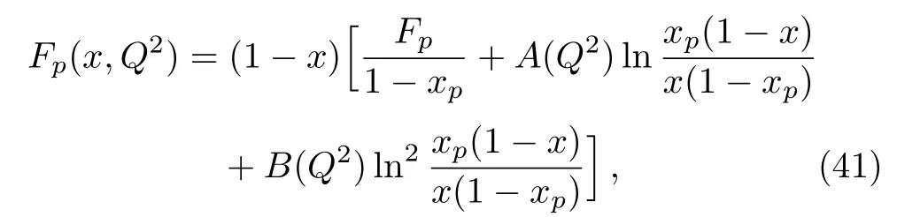


3.2 Analysis of the Gluon Distribution


4 Conclusion


 Communications in Theoretical Physics2019年1期
- Communications in Theoretical Physics的其它文章
- Impact of Colored Noise on Population Model with Allee Effect∗
- Anisotropy Effects and Observational Data on the Constraints of Evolution Dark Energy Models
- Multipolar Structure of Equilibrium Shear Flow Field in Toroidal Plasmas∗
- Dynamically Tunable and High-Contrast Graphene-Based Terahertz Electro-Optic Modulator∗
- Improved Five-Parameter Exponential-Type Potential Energy Model for Diatomic Molecules∗
- Nontrivial Effect of Time-Varying Migration on the Three Species Prey-Predator System∗