BLOW-UP PHENOMENA FOR A CLASS OF GENERALIZED DOUBLE DISPERSION EQUATIONS∗

Huafei DI(狄华斐) Yadong SHANG(尚亚东)

School of Mathematics and Information Science,Guangzhou University,Guangzhou 510006,China Key Laboratory of Mathematics and Interdisciplinary Sciences of Guangdong Higher Education Institutes,Guangzhou University,Guangzhou 510006,China E-mail:dihuafei@yeah.net;gzydshang@126.com

Abstract In this article,we study the blow-up phenomena of generalized double dispersion equations utt−uxx−uxxt+uxxxx−uxxtt=f(ux)x.Under suitable conditions on the initial data,we first establish a blow-up result for the solutions with arbitrary high initial energy,and give some upper bounds for blow-up time T∗depending on sign and size of initial energy E(0).Furthermore,a lower bound for blow-up time T∗is determined by means of a di ff erential inequality argument when blow-up occurs.

Key words double dispersion;blow up;upper bound;lower bound

1 Introduction

This article deals with the initial boundary value problem for the following generalized double dispersion equations

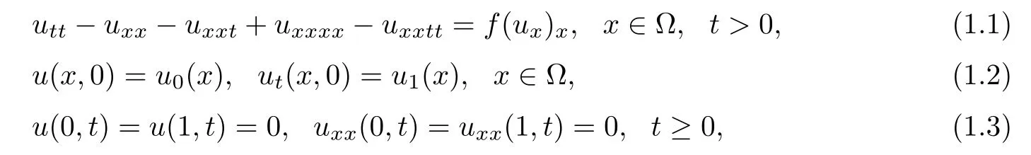
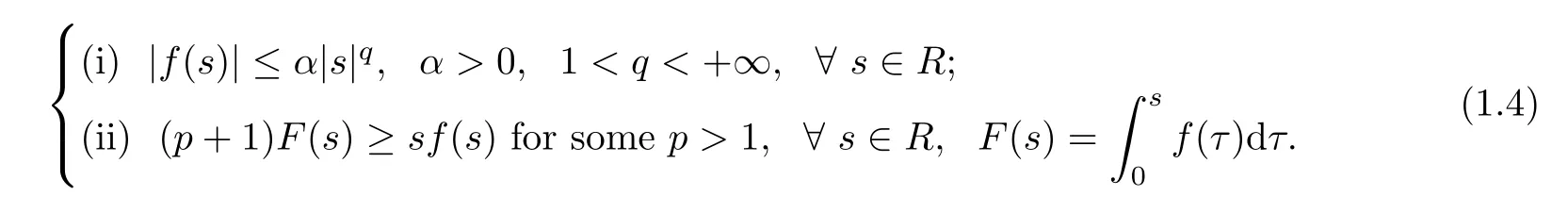
where u(x,t)denotes the unknown function,u0(x)and u1(x)are the initial value functions de fined on Ω=(0,1).The nonlinear smooth function f(s)satis fies the following assumptions

The reason why(1.1)is so attractive is that many famous and important physical models are closely connected with it.For example,in the study of a weakly nonlinear analysis of elasto-plastic-microstructure models for longitudinal motion of an elasto-plastic bar[1],there arises the model equation

Moreover,because of this propagation of the wave in the medium with the dissipation e ff ect,it is meaningful[2]to consider the following nonlinear wave equations with the viscous damping term

In[3],Chen and Lu studied the initial boundary value problem to the fourth-order wave equations

They proved the existence and uniqueness of the global generalized solution and the global classical solution by the Galerkin method.Furthermore,Xu,Wang,et al.[4]considered the initial boundary value problem,and proved the global existence,nonexistence of the solutions by modifying the so called concavity method under some conditions with low initial energy.Khelghati and Baghaei[5]proved that the blow-up for(1.7)occurs in finite time for arbitrary positive initial energy.When the strong damping term−uxxtof(1.7)is replaced by the weak damping term ut,Yang[6]studied the asymptotic property of the solutions,and gave some sufficient conditions of the blow-up.

A similar fourth-order nonlinear wave equation

was first derived by Zhu in the study of nonlinear wave in elastic rods[7],whereare constants,n is a nature number.He simpli fied(1.8)to the generalized Korteweg-de Vries-Burgers equation,and proved the existence of its solitary wave.Obviously,(1.8)is a special case of the following fourth-order wave equations

Chen[8]proved the existence and uniqueness of the global classical solutions,and gave the sufficient conditions for blow-up of the solutions to the first boundary value problem and second boundary value problem of(1.9).In[9],Chen and Hou considered the cauchy problem of(1.9).They proved the existence,uniqueness and nonexistence of global classical solutions by using the contraction mapping principle,the extension theorem and concavity methods.Chen and Guo[10]considered the asymptotic behavior and blow-up in finite time to the initial-boundary value problem of(1.9).

In[11],the authors studied the strain solitary waves in nonlinear elastic rods,there exists a longitudinal wave equation

where b0,b2are positive constants,b1is a real number,and n is a nature number.Zhang and Zhuang[12]simpli fied(1.10)to the KdV equation,and studied the existence and the qualities of its solitary wave equation.The model of(1.9)has considered the damping,so the damping term α2uxxtappears in(1.9).This is the main di ff erence between(1.9)and(1.10).More works on the higher-order wave equations can be seen in[14–23]and references cited therein.

Let us mention that(1.1)has extensive physical background and rich theoretical connotation.This type of equations can be regarded as the regularization of the fourth-order wave(1.9)by adding a dispersion term uxxxx.On the other hand,(1.1)also arises in the study of the regularization of the fourth-order wave(1.7)by adding another dispersion term uxxtt,where the nonlinear f(s)= ϕ(s)+s,s∈R.When the dispersive term uxxttof(1.1)is replaced by sixth-order term uxxxxtt,Xu,Zhang and Chen,et al.[13]considered the existence and nonexistence of global solutions to the initial boundary value problem at three di ff erent initial energy levels.In the physical study of nonlinear wave propagation in elastic waveguide,considering the model of energy exchange between the waveguide and the external medium through lateral surfaces of the waveguide,the following general cubic double dispersion equation

was derived by Samsonov,et al.[14,15]to describe the longitudinal displacement of elastic rod,where a,b,c>0 andare constants related to the Young modulus,density of waveguide,shearing modulus and poisson coefficient.

If we di ff erentiate(1.1)with respect to x and taking v=ux,it becomes the following generalized Boussinesq-type equation(n=1)

Obviously,(1.11)is a special case of the Eq.(1.12).Wang and Chen[16]considered the existence both locally and globally in time,and nonexistence of solutions for the Cauchy problem of(1.12).Chen and Wang,et al.[17]studied the existence,uniqueness of the global generalized and classical solutions for the initial boundary value problem of(1.12).

In[18–20],the Cauchy problem of the multidimensional generalization of the Eq.(1.12)

was studied.Polat and Ertas[18]proved the existence of global solutions for 1≤n≤4.Xu,liu and Yu[19]studied the global existence of weak solutions for all space-dimensions n≥1 under some assumptions on the nonlinear term and the initial data.Recently,Wang and Da[20]established the global existence and asymptotic behavior of small amplitude solution to the Cauchy problem of(1.13)for all space-dimensions n≥1.

Motivated by the above researches,in the present work we main study the blow-up phenomena for the generalized double dispersion problem(1.1)–(1.3).Currently,there are few results for the initial boundary value problem and Cauchy problem of(1.1).Many authors studied the existence,uniqueness,nonexistence and asymptotic behavior of global solutions,and have contributed to the literature for(1.1).We also refer the reader to see[14–17]and the articles cited therein.To our knowledge,there is little information on the bounds for blow-up time to problem(1.1)–(1.3).Especially,the appearance of the nonlinear term f(ux)x,double dispersion terms uxxxx,uxxttand strong damping term uxxtof(1.1)cause some difficulties in the way of the proof,when we consider the bounds of blow-up time of the solutions.Hence,we have to invent some new methods and skills to determine the upper and lower bounds of blow-up time for generalized double dispersion problem(1.1)–(1.3).

This article is organized as follows.In Section 2,we introduce some notations,functionals and important lemmas which are needed for our work.In Section 3,we establish a blow-up result of the solutions with arbitrary high initial energy,and give some upper bounds for blowup time T∗depending on the sign and size of initial energy E(0).In Section 4,we determine a lower bound on blow-up time T∗if blow up occurs to the initial boundary value problem(1.1)–(1.3)by means of a di ff erential inequality technique.

2 Preliminaries

In this section,we give some notations,functionals and important lemmas in order to state the main results of this article.

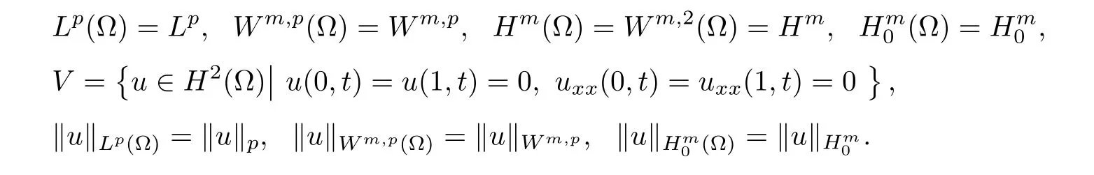
Throughout this article,the following abbreviations are used for precise statement:

Firstly,we start with the following existence and uniqueness of local solution for problem(1.1)–(1.3)which can be obtained by Faedo-Galerkin methods.The interested reader is referred to[17,24]for details.

Theorem 2.1Assume that(1.4)hold andThen,the problem(1.1)–(1.3)has a unique local solution

for some T>0.

From the Theorem 2.1,it is easy to verify that the functions ut,uxexist almost everywhere on Ω=(0,1).In addition,the combination of assumption conditions(1.4)and the existence of ux(after possibly being rede fined on a set of measure zero)ensure that the functionals F(ux)anddx make sense.

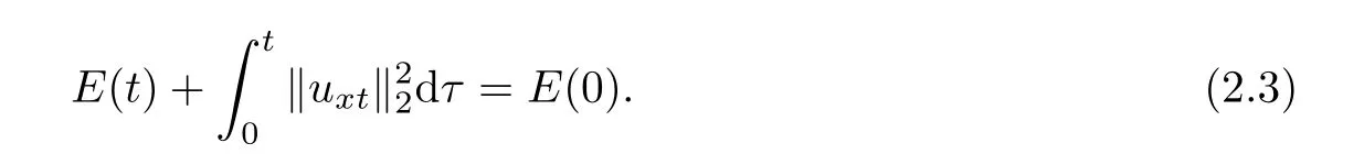
Hence,we de fine the energy functional for the solution u of problem(1.1)–(1.3)by

Then,multiplying(1.1)by utand integrating over Ω,we easily obtain

and

Next,we will mention some important lemmas which are similar to the lemmas of[25,26]with slight modi fication.

Lemma 2.2Let δ>0 and b(t)be a nonnegative C2-function satisfying

If

ProofLet r1be the largest root of(2.6).Then(2.4)is equivalent to

Multiplying e−r1ton two sides of inequality(2.7),then we have

Integrating(2.8)from 0 to t for∀k0≥0 we have

From the combination of(2.5)and(2.9),it easily obtainfor all t>0. ?

Lemma 2.3(see[25]) If J(t)is nonincreasing function on[t0,∞),t0≥ 0,and satis fies the di ff erential inequality

where a>0 and b∈R,then there exists a finite positive number T∗such that

And an upper bound for T∗is estimate,respectively,in the following cases:

(ii)when b=0,then

(iii)when b>0,then

3 Upper Bound for Blow-up Time

In this section,we give a blow-up result for the solutions with arbitrary high initial energy and some upper bounds for blow-up time T∗depending on the sign and size of initial energy E(0)for the problem(1.1)–(1.3).

To obtain the blow-up result and upper bounds,we first de fine functional

and then give the following lemma.

Lemma 3.1Let u be the solution of problem(1.1)–(1.3),and f satis fies the assumptions(1.4).Furthermore assume thatand

then the following inequality holds

ProofFrom(3.1),a direct computation yields

and

By(1.1)and(3.4),we obtain

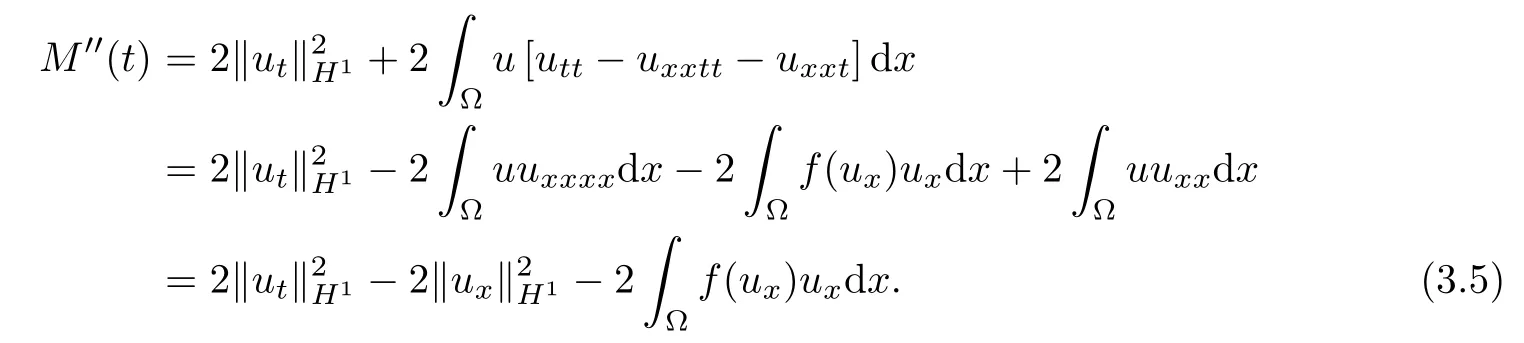
Then,using(1.4)(ii)and(2.3),it follows that

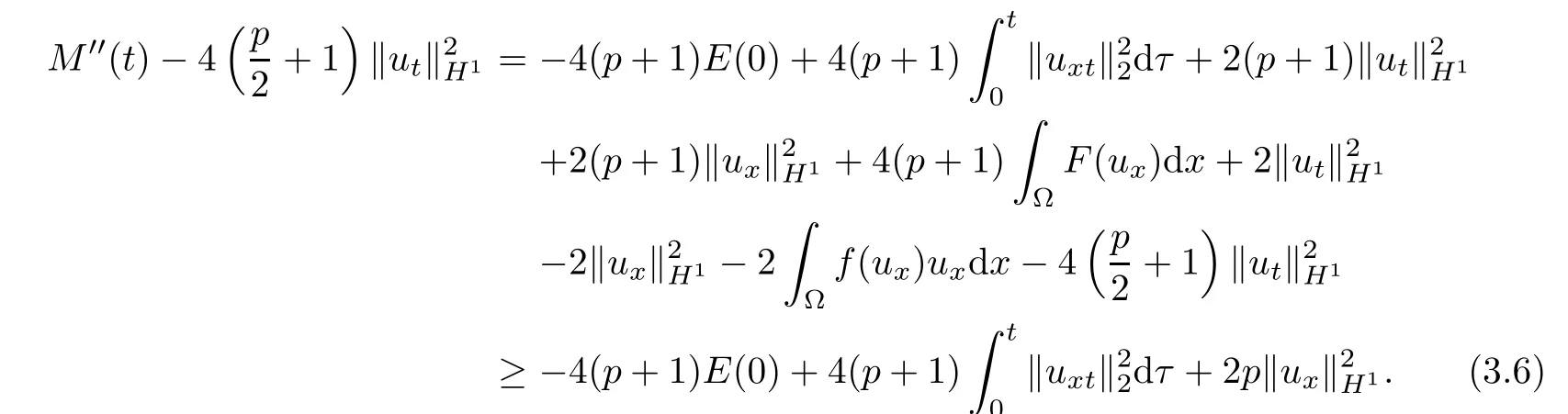
We note that

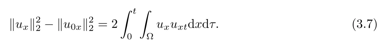
Utilizing Young’s inequality,it follows from(3.3)and(3.7)that

In view of(3.6)and(3.8),we have

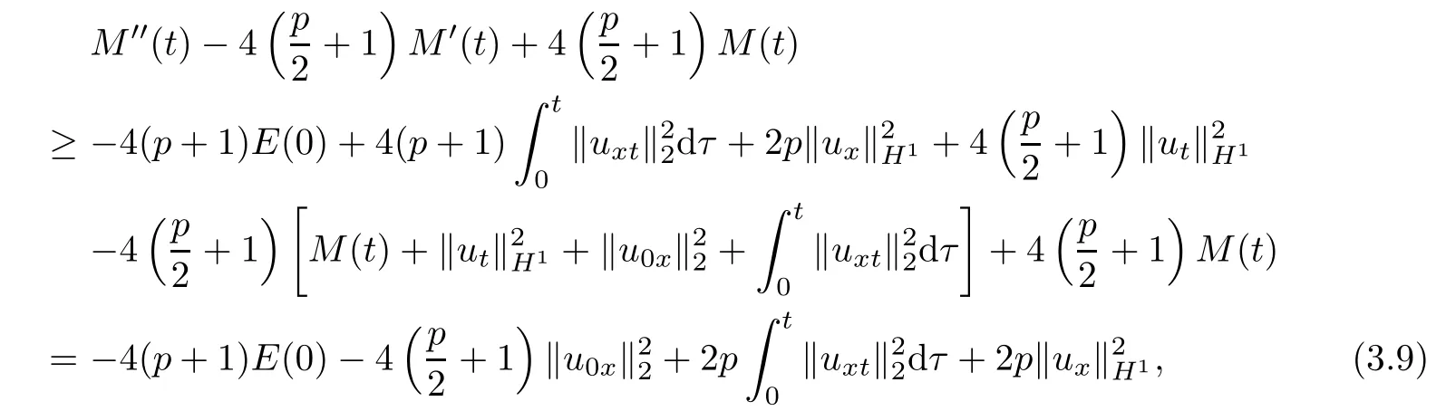
which means that

where

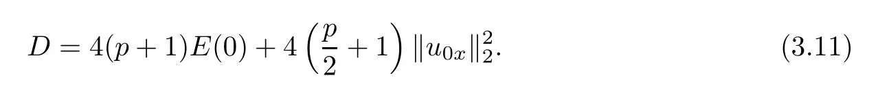
Next,we de fine

From the combination of(3.10)and(3.12),we have

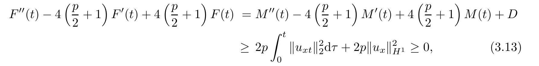
which satis fies the assumption condition(2.4)of Lemma 2.2.Then,by Lemma 2.2,we can obtain that if

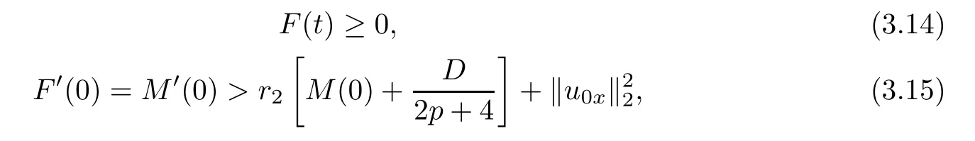
then

Furthermore,utilizing assumption condition(3.2),

and(3.16)that M(t)is increasing function,it is easy to obtain

On the other hand,by the combination of(3.11)and assumption condition(3.2),

we also make sure that the inequality(3.15)holds.Thus,the proof is completed.

Next,we shall state and prove the finite time blow-up result with arbitrary high initial energy.

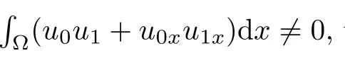
Theorem 3.2Let u be the solution of the problem(1.1)–(1.3),and f satis fies the assumptions(1.4).Furthermore assume that u0∈ W1,q+1(Ω)∩V,and

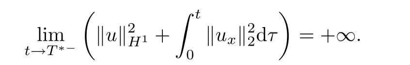
then the solutions u(t)of the problem(1.1)–(1.3)blow up in finite time,that is,the maximum existence time T∗of u(t)is finite,and

Moreover,the supper bounds for blow time T∗can be estimated according to the sign and size of energy E(0).

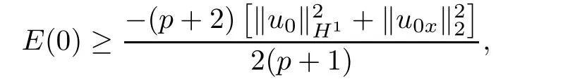
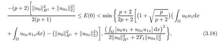
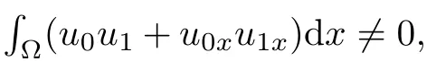
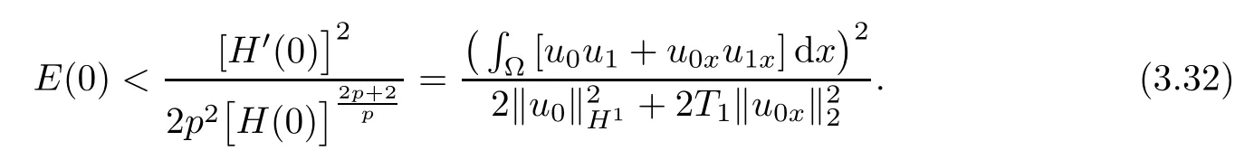
Case 1If

and inequality(3.18)holds,then an upper bound of blow-up time T∗is given by

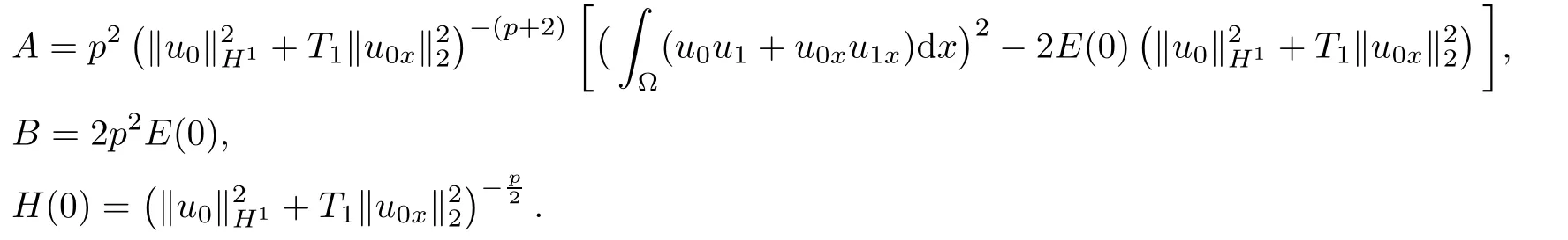
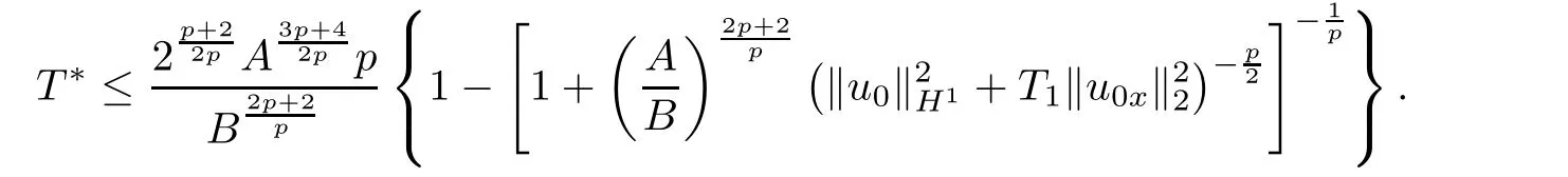
Case 3If E(0)>0 and inequality(3.18)holds,then an upper bound of blow-up time T∗is given by

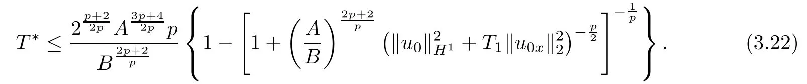
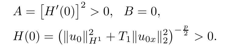
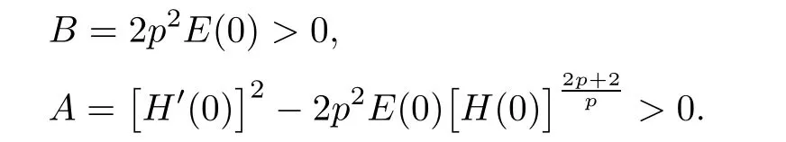
Here

ProofWe de fine functional

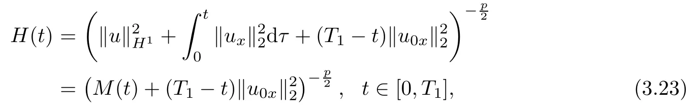
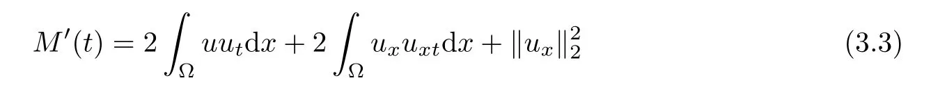
where T1>0 is a certain constant which will be speci fied later.By simple calculation,we have

and

where

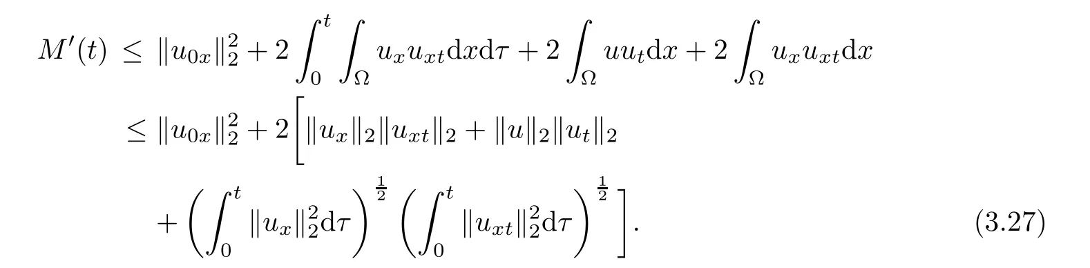
From(3.3),(3.7)and Hölder inequality,we obtain

By(3.6),we have

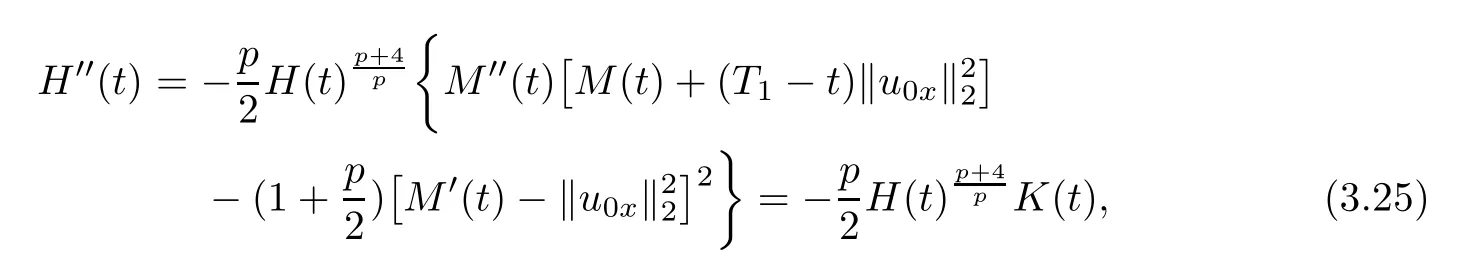
Inserting(3.1),(3.27)and(3.28)into(3.26),it follows that

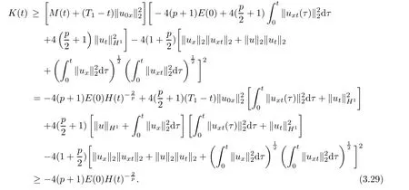
By(3.25)and(3.29),we obtain

From Lemma 3.1 and(3.24),we know that H′(t)<0 for t ≥ 0.Multiplying(3.30)with H′(t)and integrating it from 0 to t,then we have

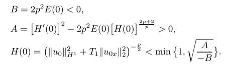
where

and

which means that

By the combination of(3.2),(3.31)and(3.32),we can obtain from Lemma 2.3 that there exists a finite time T∗such thatwhich implies that

Furthermore,an upper bound for T∗will be estimated,respectively,in the following cases:

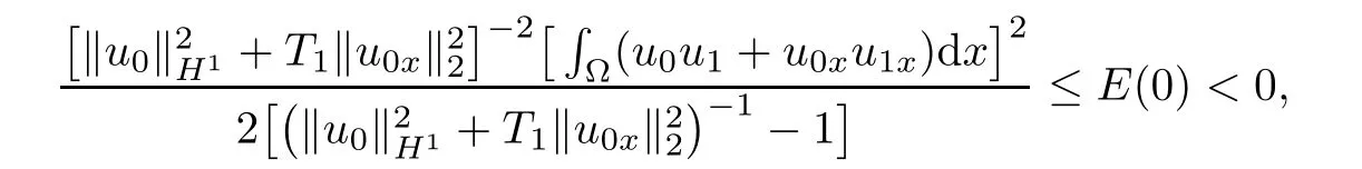
Case 1If

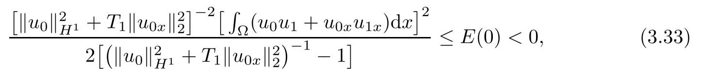
and inequality(3.18)holds,then by simple calculation,we have

Hence,from Lemma 2.3(i),it follows that an upper bound of blow-up time T∗is given by

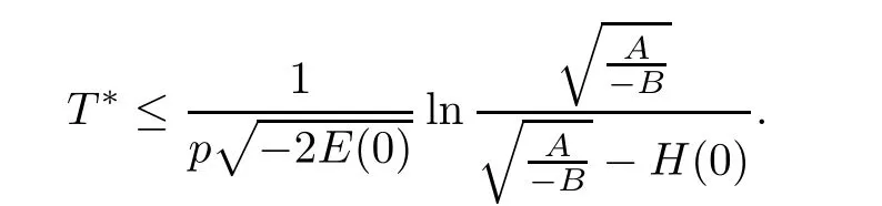
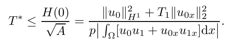
Hence,from Lemma 2.3(ii),it follows that an upper bound of blow-up time T∗is given by

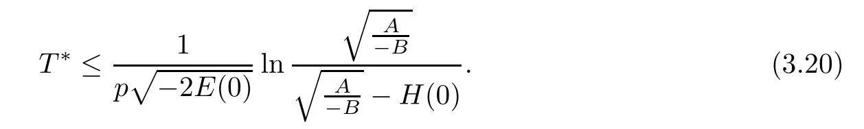
Case 3If E(0)>0 and inequality(3.18)holds,then we have

Hence,from Lemma 2.3(iii),it follows that an upper bound of blow-up time T∗is given by

Here,we choose T1≥T∗such that(3.23)is possible.Thus,the proof is completed.

4 Lower Bound for Blow-up Time

In this section,our aim is to determine a lower bound forblow-up time T∗when blow up occurs to the initial boundary problem(1.1)–(1.3).

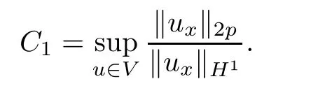
Theorem 4.1Let u be a blow-up solution of problem(1.1)–(1.3),and u0∈ W1,q+1(Ω)∩Furthermore assume that f satis fies conditions(1.4).Then,a lower bound for blow up time T∗can be estimated by

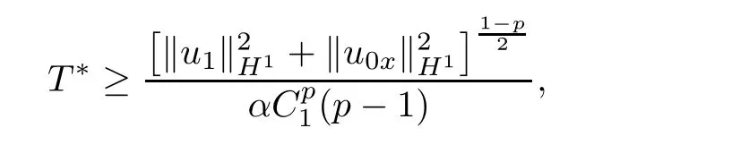
where C1is the optimal constants satisfying the inequalities kuxk2p≤C1kuxkH1.

ProofWe de fine the auxiliary function

Di ff erentiating(4.1)with respect to t and integrating by parts,then we have

Making use of the Schwarz inequality and(1.4),we have

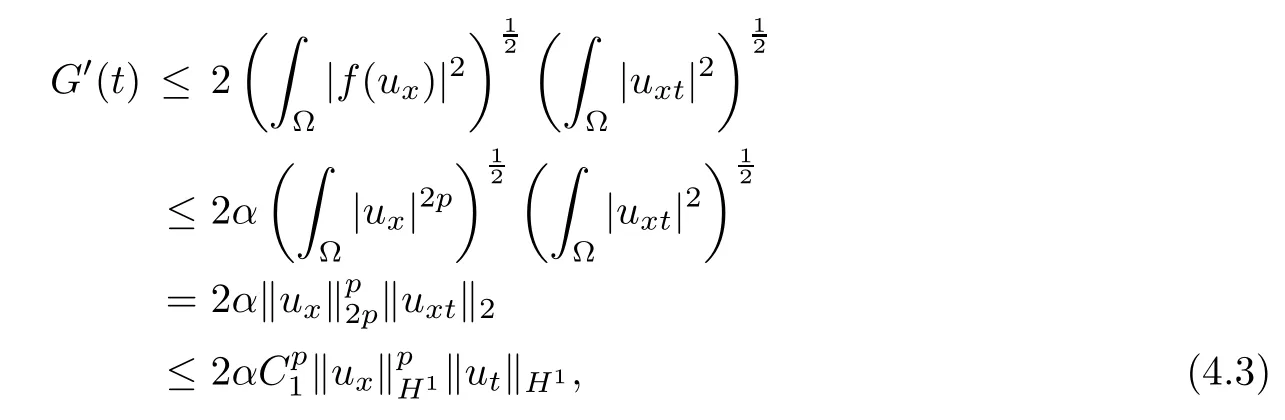
where

From the de finition of G(t),it follows that

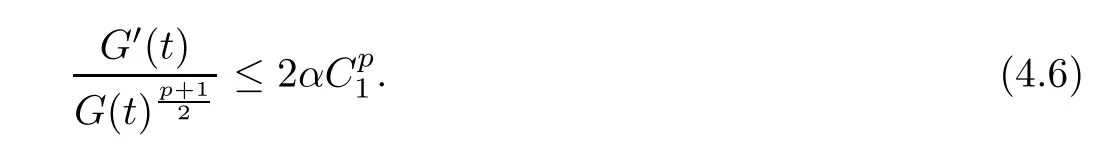
Inserting(4.4)into(4.3),we obtain the di ff erential inequality

If there exists t0∈ [0,T∗)such that G(t0)=0,then we can obtain G(T∗)=0.This contradicts with the fact that u(x,t))blows up at finite time T∗.Hence,we see that G(t)>0 and the following inequality holds

Integrating(4.6)with respect to t,then we have

So letting t→T∗in(4.7),we can conclude that

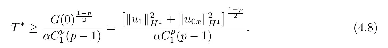
This completes the proof of Theorem 4.1. ?

AcknowledgementsDr.Huafei DI also specially appreciates Prof.Yue LIU for his invitation of visit to UTA.