
PRF: a process-RAM-feedback performance model to revealbottlenecks and propose optimizations①
2020-10-09 07:38XieZhenTanGuangmingLiuWeifengSunNinghui
High Technology Letters 2020年3期
Xie Zhen(谢 震)②, Tan Guangming, Liu Weifeng , Sun Ninghui
(*Key Laboratory of Computer Architecture, Institute of Computing Technology, Chinese Academy of Sciences, Beijing 100190, P.R.China) (* *University of Chinese Academy of Sciences, Beijing 100190, P.R.China) (* * *College of Information Science and Engineering, China University of Petroleum, Beijing 102249, P.R.China)
Abstract
Key words: performance model, feedback optimization, convolution, sparse matrix-vector multiplication, sn-sweep
0 Introduction
In recent decades, modeling has been employed to optimize performance of computational kernel and verify the validity of proposed optimization methods[1-4]. Depending on whether the model uses hardware and software features as a reference, it can be roughly divided into 2 categories. One is ‘black box’ model that uses a fitting or machine learning method to predict the performance by extracting characteristics of the target machine and collecting data of application. This method collects a large amount of application data to build a model by statistics or mathematical model. The model is not universal and does not reflect the real implementation inside architecture. The other is ‘white box’ model, which uses a simplified machine model to describe the matching relationship between application and hardware. The simplest white-box model was the Roofline model proposed by Ilic et al.[5], which can be used to bound floating-point performance with a function of machine peak performance, peak bandwidth and arithmetic intensity. However, the Roofline model cannot describe detailed bottlenecks beyond memory bandwidth and peak performance. It only shows the upper limits of the performance. A more detailed machine model with memory hierarchy was the execution-cache-memory (ECM) model proposed by Datta et al.[6]. Based on ECM model, stencil[7]loop kernel[8]and microbenchmark[9,10]have been modeled and optimized. It divides the machine into in-core and out-core phase, and reflects the time of instruction execution on processor core and data transfer between cache and memory by an address-based cache simulator (pycachesim) or proportion analysis by Kerncraft[11]. But mapping real application to address sequence requires a medium and none of these tools have yet been provided. Also this model ignores the impact for possible occurrence of data dependence and the differences between regular and irregular memory access. So it cannot accurately predict performance when the application has pipeline stall and stride or random memory access. Therefore, it cannot give specific feedback based on the incomplete information.Moreover, for specific applications, optimization methods are very different with different instructions and data sizes, the existing models cannot give fine-grained optimization guidance. In addition, there have been many work based on hardware performance counters[12-15]. Although these methods can also obtain the load characteristics by the number of monitored events, they need to monitor at runtime with unacceptable overhead.
This paper proposes a new performance model called process-RAM-feedback (PRF). It deeply considers the diversities of the pipeline and the cache layers as a ‘white box’ model. So that it can predict the instruction overhead and the cache misses for regular, irregular and data dependence applications. In this sense, the proposed model largely broadens the application domain of performance modeling. More importantly, the proposed model can give feedback guidance for the optimization, which is not available in existing performance models. In order to realize this functionality, the proposed model consists of 3 fundamental steps. Firstly, the proposed model abstracts the important hardware parameters, such as the calculation unit, access unit, instruction cost, the associativity and the size of each memory level (cache and DRAM). Secondly, based on these parameters, this paper constructs a directed acyclic graph (DAG) to predict instruction overhead and a cache simulator to predict the cache miss as the overhead of data transmission. Lastly, the proposed model can use the obtained information in the previous 2 steps, reveal the bottlenecks, compare the effects of different optimization methods, and then provide optimization guidances. In this way, the optimized kernels are obtained. This work’s main contribution is reflected in 3 aspects.
1) In the proposed PRF model, this paper considers comprehensive factors which may affect the kernel performance, e.g., the probability of instruction pipeline stall and cache line transmission between different levels of RAM, and the execution time of instructions for both calculation and memory access. Based on the theoretical and model-based analysis for specific cases, the proposed model can produce a much more accurate performance prediction and extend the application domain to the context of irregular memory access and data dependency issues.
2) In order to get the number of cache misses at all cache layers for irregular case, this paper develops a multi-level cache simulator which can be easily built on the target hardware and quickly get the needed information for the specific kernels. As an indicator of data transmission, improvement of prediction accuracy for cache miss is a crucial factor which affects the accuracy of performance prediction in the proposed model.
3) According to the different performance bottlenecks, the proposed model feeds back developers to select the best optimization method and informs performance expectation with various data inputs, instructions support and data sizes.
From regular memory access to irregular and data dependence, this paper selects 3 cases (convolution, sparse matrix-vector multiplication and sn-sweep) to verify the correctness of the model. The experiments show that, for modeling the convolution algorithm as the regular case, the PRF model could feed back the best optimization suggestion for various data sizes under current instruction support.For the irregular memory access, by running SpMV with 3 673 sparse matrices from the Florida collection[16], the average error rate: ABS(predicted_value-measured_value) / measured_value of PRF model is about quarter than the ECM model. Further, for sparse matrices, feedback optimization guides developer to select the parameter (i.e., block size) for the block compressed sparse row (CSR) sparse matrix format by using the output of the PRF model and it highly matches the best block size manually selected from exhaustive experiments. As for sn-sweep, PRF model constructs the DAG through its calculation process, and analyzes the data dependency relationship between instructions to reveal the problem of pipeline with out-of-order execution support, and finally guides to solve data dependence issue and its performance improvement is about 192% in single-core pipeline with linear scalability for multi-core.
1 Related work
Performance modeling is a very useful technique for optimization of parallel applications on high performance computing (HPC) platforms. All of the current architecture can be divided into the instruction part and the memory part. As shown in Fig.1, it results different abstract methods can build various performance models. Next this paper begins to introduce the differences between 4 performance models.
The Roofline[5]model is a visual analytical model used to pinpoint performance bottlenecks. For the instruction part, the Roofline model abstracts it as a black box, this model describes the peak computing performance as the upper limit of the instruction part, which constraints the best performance of which program can achieve. Same as before, the Roofline model also abstracts memory part as the peak memory bandwidth. It can also be applied to any program. However, the model gives little detail information, and lacks accuracy of performance prediction for target application.

Fig.1 PRF model and comparison with Roofline, cache-aware Roofline and ECM
As a refined model on Roofline, cache-aware Roofline[17]joins the implications of the cache hierarchy, and the transmission bandwidths of cache are used as boundaries. But this model has the same disadvantages as Roofline by low accuracy.
The ECM[6]model considers the time for executing the instructions with data coming from the L1 cache as well as the time for moving the required cache lines (CLs) through the cache hierarchy. It also calculates the time for executing instructions of loop kernel on the processor core (assuming no cache miss) and transferring data between its initial location and the L1 cache. The in-core execution time T_core is determined by the unit that takes the most cycles to execute the instructions. The time needed for all data transfers required to execute one work unit is expressed as T_trans. The in-core execution and transfer costs must be put together to arrive at a prediction of single-thread execution time. By simulating execution of CPU instruction, the model has a good prediction accuracy for regular memory access pattern. But ECM could predict performance in the memory part of a sort, it divides memory part into an undifferentiated cache layer and main memory, making it hard to model data locality.
Therefore, for irregular application, these 3 models are difficult to give accurate prediction, and the error mainly occurs in the memory access phase, and there is a considerable gap between the size of data transfer and the data reuse of irregular application by these model predicts and real situation. Also the ECM model ignores the effect of pipeline stall. This is also the main focus of the proposed model. Here this paper realizes a pipeline DAG with more realistic memory hierarchy, and designs a cache simulator to output approximately real cache miss for irregular case. With the abstract method, PRF model can achieve better predictive accuracy, while also covering more irregular and data dependence cases. The comparison of all models is shown in Fig.1.
Cache simulation has been used to evaluate memory systems for decades. Fei et al.[18]examined the topic for multiprocessor memory-systems. Liu et al.[19]investigated an x86 cache simulation framework in the specific context of multiprocessor systems. Llatser et al.[20]discussed many intersection properties for caches using different replacement policies, and Dey et al.[21]studied coherency protocols between different caches in a shared memory system. These simulators are constructed by configurations, such as cache size, sets, cache associativity, block size, replacement policy according to a specific application. However, for program optimization, these cache or memory simulators are not efficient enough since the cost for lots of hardware emulation functions. Thus applying them in real-world applications will lead to new performance bottlenecks. This paper designs a light weight cache simulator that can simulate all levels of cache miss with a very low overhead for all memory access patterns.
As for regular memory access pattern, convolution operation in convolution neural networks is the most time-consuming function. Brechet et al.[22,23]used the vectorization instruction or designed the unique hardware structure to speed up the calculation, but this optimization is case by case, since the effective optimization method for different data sizes and machine structures is quite different, so the proposed model is to find a set of methods to optimize the regular memory access applications in different architectures and guides the developer to obtain higher performance.
Sparse matrix-vector (SpMV,y=Ax) multiplication is an important computational kernel with an irregular memory access patterns. The SpMV operation does not contain any dependencies and has relatively high parallelism. Buttari et al.[24]used a modeling method to optimize the SpMV by blocking. But this model fits machine characteristics and predicts performance by fill-in the dense matrix to achieve the best block sizes. Li et al.[25]used register-level tiling opportunities to select parameters for BCSR by model. However, these parameters tuning are time-consuming and none of these methods can reflect real execution on the current architecture of SpMV. Then this paper quantifies instruction and memory transmission for various parameters, and selects the best block size and predicts optimized performance.
Sn-sweep is a typical regular application with very low performance as data dependence. It is the largest time-consuming function for numerical simulation of radiation transport in high energy density plasma physics[26]. As sn-sweep can be seen sweep the radiation flux from the source across the grid in the downstream direction, so grid decomposition method makes task parallelization easier. Liu et al.[27]described message passing implementations of sn-sweep algorithms within a radiation transport package to increase expandability. The proposed model focuses on bottlenecks within a task and exposes the cause of the instruction pipeline stall to guide optimization.
2 The PRF performance model
The PRF divides model into 3 parts: process phase, RAM phase and feedback optimization phase. The process phase corresponds to the instruction part, which predicts the cost cycles within the CPU core by executing internal instruction with pipeline, while the RAM phase corresponds to the memory part, which describes the connected relationship and predicts the time between memory hierarchy. The feedback optimization phase collects the output of each phase, analyzes execution bottlenecks and potential opportunities, and provides developer optimization guidance. In Fig.2, this paper visualizes these 3 phases, and sets the time of process phase when all instructions and datas are in the L1 cache, the time of RAM phase is the transfer time between the memory hierarchies. The outputs of model are evaluated, analyzed and directed by feedback optimization phase.

Fig.2 Three components and workflow of the PRF model
For process phase, this paper first divides the instruction into computation instruction and memory access instruction, and builds a DAG to describe data dependencies. Through the implementation of the pipeline, it outputs the overhead for 2 kinds of instructions. Then this paper labels the cost time of calculation and memory access instruction as T1 and T2. For the RAM phase, due to the principle of locality, different inputs and applications will result in different cache miss, so memory access instruction does not definitely cause datas transfer (if datas are in cache). Also this paper founds that the current Intel processors have a prefetching mechanism for the regular memory access, resulting in almost no cache miss at some cache levels. So this paper separates the regular and irregular data, and the time of transmission for regular data can be calculated by format which will be described in detail later, and also builds a multi-level cache simulator for irregular data, then simulator can output the number of cache misses at all levels. Therefore this paper can obtain the time of all the data transfer and label the transmission time of 3-level cache as T3, T4, and T5. The feedback optimization phase abstracts 4 performance bottlenecks, uses the output of the model to point out the key factors which affects performance most, and guides developer to improve performance which optimization can bring.
2.1 Process phase
Instruction is mainly divided into 2 types: computation (addition and multiplication) and memory access (load and store) instruction. The 2 kinds of instructions are scheduled independently in core internal and can properly implement instruction-level parallelism without data dependence. Although current processor has out-of-order execution mechanism, when data dependency occurs, the instruction which depends on the previous results will also cause performance stall[28].
In order to model the pipeline, this paper designs a DAG module, which is constructed as shown in the Fig.3. It uses a blank circle representing read without write, a solid line with an arrow representing the direction and load a data, and the grid circle representing read after write. By analyzing the code of an application to build the DAG, execution flow of the DAG shows pipeline analysis of data dependence. For example, on a 3-stage pipeline processor, R3 occurs data dependence for read after write, resulting in one stall for data dependence.

Fig.3 DAG for modeling data dependence
As an example, this paper builds the PRF model on an Intel Haswell architecture. This microarchitecture can execute one addition and one multiplication operation or 2 fused multiply add (FMA) operations per cycle, while supporting 2 load operations and one store operation per cycle. All details will be introduced in the Section 3. So if the numbers of addition, multiplication, FMA, load and store instruction are A, M, FMA, L and S respectively for an application, then the time spent on process phase can be calculated by Eq.(1).
T(processphase)
(1)
2.2 RAM phase
RAM phase converts cost of data transmission into overhead between each level of cache and main memory. As the size of each level of memory hierarchies are very different for various architectures, data may appear in any of them, resulting in complicated data transfer time. When a CPU requests memory access, it will seek a data block as cache line from L1, L2 and L3 caches to main memory in turn. If the former search is missing, this cache line will transfer from the lower level of memory hierarchy to the upper level. At the same time, the current cache has a perfect prefetching mechanism for the regular memory access, resulting in a significant reduction in transmission time.
Therefore, as in Fig.2, RAM phase model partitions memory accesses into regular and irregular memory access. For regular memory access, it is to access continuous memory address or cache line, or visit fixed stride memory address. For the Haswell core this paper used to model, the L1 cache cannot implement prefetching operation as the first level of cache by lots of experiments. Then for other cache levels, when data is read from L2 cache to L1 cache, the adjacent data which will be accessed is transferred from L3 cache to L2 cache, and since the transmission bandwidth of L3 to L2 is half than L2 to L1, it leads to a half overlap. At the same time, other adjacent data which will be accessed is transferred from the main memory to L3 cache, and the bandwidth of main memory to L3 is lower than the cache, so there will be a delay by the differences.
Assuming that the internal bandwidth of cache which data appear isC, the bandwidth between the main memory and the last level cache isM, and the regular data size to be accessed isAmount_regular, the time spent on regular memory access pattern is given in Eq.(2).
T(RAM_phase_for_regular)
(2)
For irregular memory access, cache prefetcher cannot work well when accessing disordered address, the data which needs to be accessed may appear on any of the memory hierarchy, so loading these irregular data will produce unexpected cache misses. In order to get these cache misses, this paper designs a cache simulator, which could simulate cache groups and cache lines, and use index number (similar to the address) to distinguish each cache line. Then the simulator builds memory access sequence based on the user’s input data and memory access process, and finally outputs cache misses. It also simulates the replacement mechanism.
Unfortunately, the Intel smart cache replacement policy is confidential, so this paper carries out a large number of experiments and obtains some conclusions: L1 cache uses least recently used (LRU) policy, L2 and L3 are based on the LRU policy with relatively perfect prefetching operation for regular memory access.
Therefore, the process of building the cache simulator can be described as follows. (1) Detect the size and group associative of the cache at all levels, and assign corresponding tags which could mark block number and valid bit. (2) Build the mapping relationship at all levels. (3) Set its replacement strategy.
The internal work-flow of the cache simulator is as follows. (1) Detect current physical machine and build the cache simulator. (2) Partition the input data which will be accessed to corresponding cache lines and mark it as regular or irregular. (3) The cache simulator reads cache lines by marking the cache block valid nor not, prefetchs regular cache lines and records the miss numbers. (4) Finally, through the known data transfer rate, the cache simulator will output cache miss and cost at any of the memory hierarchy. If the 3 cache misses is L1_miss, L2_miss and L3_miss respectively and the size of cache line is CL, the time spent is given in Eq.(3).
T(RAM_phase_for_irregular)
(3)
The sum of process part and RAM part shows the overall completion time of the program. It can be calculated by Eq.(4). And giga floating-point operations per second (GFLOPS) can be calculated by Eq.(5).
T(PRF)=T(process_phase+RAM_phase-overlap)
+T(RAM_phase))
+T(RAM_for_regular)
+T(RAM_for_irregular))
(4)
GFLOPS(PRF)
=(A+M)×CPU_Frequency/T(PRF)
(5)
2.3 Feedback optimization phase
According to Fig.2 and Eq.(4), this paper splits the time for each stage from T1 to T5.As shown in Fig.4, the abscissa indicates the data size, and the ordinate indicates the GFLOPS. The line T1 represents floating-point performance without memory access time, and the line (T2+T3+T4+T5) represents floating-point performance without calculation time. So the final execution time is the minimum value of line T1 and line (T2+T3+T4+T5). This paper enumerates 4 different possibilities and shows how to discover the bottleneck and optimized code.

Fig.4 Four different optimization opportunities
As shown in Fig.4(a), it can be observed the line T1 cannot reach scalar peak performance without data transmission, so feedback optimization guide developer to choice intermediate variable to reduce the data dependence for addition and multiplication operation. Then the arrow represents the reduction of T1 and improvement of GFLOPS by decreasing the time of calculation instruction. Through the changes of feedback optimization, the line with cycle performance line can be upgraded to the line with triangle performance line with the data size increasing. As same for Fig.4(b), the line T1 cannot reach floating point peak performance without data transmission, so feedback optimization guide developer to choice the single instruction multiple data (SIMD) to increase calculation speed. If T2 has spent much more time and become a bottleneck, it presents the data access instruction that has become worthwhile optimization. Feedback optimization informs developer to redesign data structure or increase the redundant space to reduce the time of memory access instruction, and the optimization effect is shown in the Fig.4(c). If this paper finds that the memory access part is bottleneck, then feedback optimization will warn developer to increase cache utilization and reduce the transmission time by using new data format or cache-based block design in the Fig.4(d).
Next, this paper will use 3 cases to implement the whole process of modeling.
3 Experimental testbed
This paper uses an Intel Xeon E5-2680 v3 processor[29]with the SSE, AVX and AVX2 support for validating the proposed model. Each core can execute one multiply and one addition in floating point or 2 FMA instructions per cycle without data dependency. The memory hierarchy consists of 3 on-chip SRAM data caches. For the scalar instruction[30], the memory read and write instruction (load and store) is only one kind, and the data is always aligned. For the vector instruction, memory access instruction is divided into load, loadu, store and storeu by respectively accessing aligned and unaligned data, and the time spend on unaligned data is twice as large as for aligned data. All the specifications are listed in Table 1.

Table 1 Special machine parameters
4 Validation
4.1 Convolution
4.1.1 Convolution operation
Convolution operations have been widely used in denoising, extraction, structure smoothing, filtering, detection, image enhancement and many other image processing applications. The information of images is encoded in the spatial domain rather than the frequency domain, thus the image convolution operation is extremely essential and useful in image processing. For real-world applications, 32 bit floating point is usually selected for rapid training. For 1D convolution, the convolution filter is a 1-dimension structure, as horizontal filter with size of 1×N. 1D convolution operation simply rotates the convolution kernel 180 degrees before multiplying the input data. Fig.5 illustrates anm×ninput data convolved with a 1×16 kernel size and its DAG. Each pixel in the window is multiplied by their corresponding kernel coefficients and finally generate the whole output data.
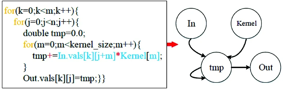
Fig.5 DAG of 1D convolution
4.1.2 Performance prediction for naive code
From the proposed example, it can be seen that the 1D convolution requires reading 16 kernel data and 16 input data to perform 16 addition and multiplication calculations. This paper can easily find out data is reuse access, along one dimension for 1D convolution. The next iteration operation will reuse 15 elements from the previous iterations.
For this program, the kernel array has good locality, and it can always be stored in L1 cache. Reading a cache line of in and out data separately will update 16 values of out, and contains both 16×16 addition and multiplication instructions, and therefore it also produces 16×16 load and 16 store instructions. For the current architecture, each cycle can execute an add and mul instruction, so the cost cycle of all of those addition and multiplication instructions is 16×16=256, and a cycle can perform two load instructions and one store instruction. So the cost cycle of access instruction is 256/2=128, For L2->L1 and L3->L2, a cycle can transfer one cache line and half of a cache line respectively, namely data transmission requires 1 or 2 cycles for a cache line, For MEM->L3, a cycle can transmit 1/5 cache line, finally this paper can infer the GFLOPS performance in different data sizes which are shown in Table 2, for example, the GFLOSP=(16×16×2)/(max(256,128+2/4/10)/2.7) Gflops.

Table 2 GFLOPS performance in different data sizes for naive code, and comparison
From the performance analysis given above, it can be seen that, regardless of the data at any memory hierarchy, the largest cost of a 1D convolution is the computational instruction (T1). Next, this paper will introduce different optimization methods, and analyze the optimized performance.
4.1.3 Optimization method and modeling analysis
By comparing the overhead of each phase, this paper can see that the T1 becomes a bottleneck. From the Fig.4, the performance reaches the scalar peak which means there is no data dependence in the calculation process, so the optimal GFLOPS can be achieved when using SIMD by feedback optimization phase in Fig.4(b). For the current machine platform, it supports SSE for 128 bit and AVX2 for 256 bit. So this paper will implement optimized version for AVX2 instruction with unaligned data and give the performance prediction. The pseudo-code is given in Algorithm 1.

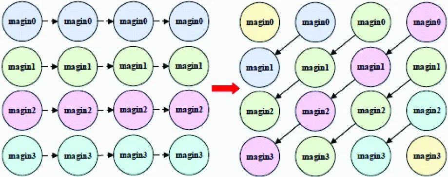
Algorithm 1 AVX2 unroll unalignedInput: IN[], length, KERNEL[], kernellength;Output: OUT[]Input: IN[], length, KERNEL[], kernellength;Output: OUT[]1: m256 kernelreverse[kernellength](aligned);2: for i=0; i For 16 iterations of the program, it will produce 16×2 addition and 16×2 multiplication instructions. It also produces 16×2 loadu and 2 storeu instructions and 7 additional addition operations. Therefore, the cost cycle of all addition and multiplication instructions is 16×2+7=39. By using AVX2 instruction and data is unaligned, the cost cycles of access instruction is 16×2×2/2=32. The GFLOPS performance is given in Table 3. Table 3 GFLOPS performance in different data sizes for naive code, and comparison 4.1.4 Optimization guidance After the previous experiments, this paper finds that the best optimization scheme depends on the supported instruction set and size of the image data set. From Fig.6, this paper extends to predict performance from SSE to AVX2 with aligned memory access or not for different data sizes. Then this paper can clearly observe that the SSE instruction set can achieve good scalability. When using the AVX2 instruction set, data transmission begins to affect performance with the increase of data size, then there is no way to achieve the peak of floating-point calculation, therefore, using AVX2 instruction set cannot linearly improve performance. As aligned memory access needs addition data storage, the method is only efficient with a small amount of data size. So the feedback guideline recommend developer to use vector instruction with unaligned access and increase the memory transmission optimization with AVX2 support. Fig.6 Modeling and prediction of various instruction In this section, this paper will use 3 627 matrices in the Florida sparse matrix library[16]to verify the PRF model and compare with ECM model (as ECM releases Kerncraft and Pycachesim, so this paper could only use these 2 tools and the idea of the ECM paper as much as possible to model SpMV), find bottlenecks and propose optimization scheme. Finally, this paper chooses the optimal implementation with some randomly selected matrices. 4.2.1 Test matrices The sparse matrices this paper used to model cover all the Florida sparse matrix library. And these matrices come from a wide variety of applications with different sparse distribution characteristics. Similar to earlier work on SpMV, the CSR kernel also use row decomposition, loop unrolling and software prefetching. Some randomly selected matrices are used in previous papers[31], and the bar matrix is extracted from a real case of the actual problem. In real-world applications, 64 bit floating point is usually selected for better precision. 4.2.2 Performance prediction and bottlenecks The pseudo-code for CSR-based SpMV is given in the left of Fig.7. For process phase, this paper builds data dependence DAG on pseudo-code, and by using multiple registers, compiler can generate independence code as shown in the right of Fig.7. Then almost all instructions can execute pipeline. Fig.7 Pseudo-code and DAG for CSR-based SpMV For a sparse matrix, its row, column and nnz is R, C and NNZ, then the size of integer array A.row_ptr is (R+1)×4 Byte, the size of integer array A.col_index is NNZ×4 Byte, the size of double array A.value is NNZ×8 Byte, the size of the double array for vectorXis C×8 Byte. The red place in pseudo-code is multiplication and addition, respectively. There are NNZ ADD and NNZ MUL instructions, while the upper place indicates memory access, A.row_ptr needs (R+1) LOAD instructions, A.col_index needs NNZ LOAD instructions, A.value needs NNZ LOAD instructions, vectorXneeds NNZ LOAD instructions, the output vectorBneeds R STORE instructions, it has a total of NNZ ADD, NNZ MUL, 3×NNZ LOAD and (R+1)STORE instructions. Meanwhile, all instructions can execute pipeline. By Eq.(1), the time spent on calculation units is NNZ cycles and the time spent on memory access units is 1.5×NNZ cycles. The floating-point operations is NNZ(ADD)+NNZ(MUL)=2×NNZ. For RAM phase, the main uncertain time cost needs to model is varieties data transmission of vectorXfor kinds of sparse matrices. Then, this paper divides the data of matrix and vectors by the size of cache line and mark, as regular and irregular respectively. According to the RAM phase mentioned in Section 2, this paper builds a cache simulator by reading hardware parameters of the target machine, such as cache sizes and group associations. The simulator reads the marked data blocks in turn and records the cache misses. Therefore it simulates regular memory access of the CSR matrix with prefetching and out-of-order access of the vector. The GFLOPS of a special matrix is finally obtained by Eq.(5). As shown in Fig.8, the abscissa of all sub-graphs represents the degree of sparsity of the matrix, and it is sorted from small to large in order, and the ordinate of Fig.8(a) represents the error rate of simulated values to measured data for GFLOPS. When the real value is the same as the predicted value, the error rate is 0%, so the neighborhood of 0% represents that this model can produce fairly accuracy prediction. The ordinate of Fig.8(b), (c) and (d) represents the ratio of simulation to measured data for L1 miss, L2 miss and L3 miss and the rate of 1 represents perfect prediction. The measured L1, L2, and L3 cache misses used PAPI’s[32]statistics. Fig.8 Single core PRF model for SpMV on 3 627 sparse matrices Through the observations, for Fig.8(a), when the sparsity is less than 0.0002 or greater than 0.00045, about half of the points appears between 0.5 and 1.5 which is slightly better than ECM. When the sparsity is between 0.0002 and 0.00045, the predictions are significantly better than the ECM model, and the error rate of prediction is more than twice as small as the ECM. For sub-graph Fig.8(b), (c) and (d), it is found that most of the prediction data are concentrated near the rate of 1, which is obviously contrasted with ECM, and it is also the main reason why GFLOPS prediction accuracy is better than ECM. But there are several reasons for the predictions not to exactly agree with measurement. (1) The real cache replacement policy is unknown. (2) The actual throughput is not a constant. However, the proposed method can also achieve high prediction accuracy with Eq.(5) and cache simulator. 4.2.3 Feedback performance optimization Analyzing the performance of SpMV, this paper found that the max time and the bottleneck is (T3+T4+T5). As the CSR format matrix results in a large number of repeated data transmission of slice vectorX, by changing the format of sparse matrix, this paper can increase locality of vectorXand reduce matrix index transmission, thus it can reduce the time of data transmission and increase the efficiency of floating-point operation. So this paper randomly selects 12 matrices and one engineering matrices-bar. Through modeling, this paper finds that the CSR format causes a high L1 and L2 cache miss, then T3 is about 1.8 times than T4 and T4 is about 3.9 times than T5, resulting in a large time of data transfer. So this paper thinks of ways to optimize (T3+T4). For many solutions for cache optimization, register blocking is a typical technique for improving data reuse. The sparse matrix is logically divided into blocks and those blocks usually contain at least one non-zero. SpMV computation proceeds block-by-block. For each block, this paper can reuse the corresponding elements of the vectorXby keeping them in registers to increase temporal locality. Register blocking uses the blocked variant of compressed sparse row storage format and it is also called BCSR for short. Blocks within the same block row are stored consecutively, and the elements of each block are stored consecutively in row-major order. BCSR potentially stores fewer column indices than CSR (one per block instead of one per non-zero). The effect is to reduce memory traffic by reducing index storage overhead and reusing the vector slice. Then the T3 and T4 and even T5 can be reduced. However, a uniform block size may require filling in explicit zero values, resulting in extra computations and data traffic. Based on the above principle, the feedback optimization is implemented based on BCSR format. Now, this paper applies the PRF model to the BCSR format. By reading the matrix to cache simulator, this paper can get the cache misses and increase zero elements calculation, and finial put forward the optimal block shapes, then the partitioning scheme is given. In Fig.9, this paper models BCSR format for selected 18 Fig.9 Overall speedup of test matrices by optimization suggestion matrices, gives recommendation with an average speed-up of 173.79% and compares with hand tunning for BCSR. For the rail4284 matrix, modeling result find that the matrix does not have blocking characteristic, so traditional CSR can achieve better performance. Compared to the direct select optimal parameter by 64 SpMV time, the method greatly saves the overhead of selecting the optimal parameter by 12 SpMV time, so the model greatly improves the efficiency of feedback optimization. 4.3.1 Sn-sweep operation In particle transport simulations, radiation effects are often described by the discrete ordinates (sn) form of Boltzmann equation. In each ordinate direction, the solution is computed by sweeping the radiation flux across the grid. Sn-sweep operations have been widely used in radiation transport, radiation effect and many other high energy density plasma physics applications. For scanning algorithm, sn-sweep is an essential example of calculating the relationship between the influences of adjacent elements. The main process flow of sn-sweep is to sequentially calculate the influence of neighboring elements and update the surrounding elements. The left side of Fig.10 shows a core function of sn-sweep, it needs to multiply the left and upper elements by 2 weights and add the sum to the current element, then one iteration is to complete corresponding calculation of all the mesh. Fig.10 Pseudo-code and DAG for sn-sweep 4.3.2 Performance prediction and bottleneck analysis In the process phase, the pseudo-code is transformed into a DAG, and it is calculated by the line order in each iteration. This paper can see that when calculating the next element, the result of the previous elements must be calculated. This will lead to the pipeline stall. Fortunately, the out-of-order engine component of the current processor can only mitigate the restrict of data dependency to some extent. For this case, the calculation of an element requires 4 additions, 3 multiplications, 5 loads and 1 store instruction. Since the pipeline needs to wait for the result of previous elements, it still takes 3 cycles to get an addition or multiplication result in the worst case. In RAM phase, all data access is regular and the data is generally small, it does not cause any data transmission, so RAM phase time is 0. By Eq.(5), the worst GFLOPS is (3+4)×2.7 / max((4×3),2.5) = 1.575 Gflops and actual measurement of 1.79 Gflops with out-of-order enable. Then this paper uses ECM to model sn-sweep by Kerncraft or Intel architecture code analyzer (IACA), it predict the GFLOPS is (3+4)×2.7 / max((4×1),2.5)=4.725 Gflops with the ideal instruction throughput. The reason is the data dependencies between instructions are stored in an index_i_up array which ECM fails to find and model it. Then from Table 4, this paper extends to predict performance with different data size from L1 to MEM by PRF and ECM model. The calculation of one point requires data transfer of 5th-8th of the cache line. This paper can clearly observe that the prediction accuracy of the PRF is better than the ECM when the amount of data is less than the L3 cache size. So this paper uses the modeled time to apply the feedback optimization phase, and it can be seen that the performance cannot reach the scalar peak as the T1 takes extra time, so the model feedback pipeline is the primary bottleneck which needs to be optimized by Fig.4(a). Table 4 GFLOPS performance in different data sizes for naive code, 4.3.3 Optimization method and feedback By comparing the overhead of each phase, this paper can see that the computation instruction becomes a bottleneck, and the optimized GFLOPS can be achieved when the instruction pipeline is optimized: (3+4)×2.7 / max((4×1),2.5) = 4.725 Gflops. This paper found that there is no data dependence between the diagonal elements and that the calculation order does not affect the final result by analyzing the DAG. As shown in Fig.11, this paper improves the algorithm to optimize the instruction pipeline by using the diagonal calculation order, and rearranges partial instruction with adding some calculation of subscripts, then the optimized GFLOPS is 4.43 Gflops. Based on this optimization, this paper can continue model sn-sweep, analyze bottlenecks by feedback optimization and increase SIMD operation to boost performance. Then this paper accelerates the addition and multiplication instructions by AVX2, and achieves a certain degree of vectorization and reaches the optimal performance of 10.53 Gflops. Through the experiment, this paper finally converts a data dependence problem into memory access instruction bottleneck. At the same time, the inaccurate model prediction will affect the developer to select the corresponding optimization method, resulting in the selected method does not have any optimization effect. This discovery also shows that the bottleneck will change under different optimization methods, so this paper needs to model optimized kernel and explore more in-depth optimization. That is the meaning of feedback optimization. Fig.11 The computational order of eliminating data dependencies The PRF model is described in this paper which provides an insightful perspective to predict compute performance and to generate targeted optimization guidance. This work introduces the PRF performance model, and described in detail about the process phase, RAM phase and feedback optimization phase. Then this paper applies the model to convolution, SpMV and sn-sweep which are typical representatives of regular to irregular memory access and data dependence. It can continue to cover more applications. Table 5 compares with Roofline model and ECM model, the proposed PRF model greatly improves predict accuracy for data dependence and irregular memory access by newly designed DAG and cache simulator, and achieves comprehensive feedback ability. Table 5 Comparison with 3 performance models from different perspectives The hook indicates the model has this function, the fork represents the model does not have this function and the bar represents incomplete function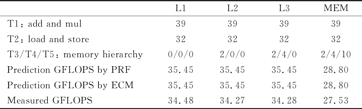

4.2 SpMV


4.3 Sn-sweep


5 Conclusion

 High Technology Letters2020年3期
- High Technology Letters的其它文章
- A novel flow control scheme for reciprocating compressorbased on adaptive predictive PID control①
- Fraud detection on payment transaction networks via graph computing and visualization①
- MSONoC: a non-blocking optical interconnection network for inter cluster communication①
- Research on full-period acquisition method for diesel enginebased on self-adaptive correlation analysis①
- Research on robust control strategy of single DOF supporting systemof MLDSB based on H∞ mixed-sensitivity Method①
- Research on oil film characteristics of piston pairin swash plate axial piston pump①