
从局部到全局的规则模型:粒聚合研究
2021-02-27 04:50PEDRYCZWitold
同济大学学报(自然科学版) 2021年1期
PEDRYCZ Witold
(加拿大阿尔伯塔大学埃德蒙顿分校电气与计算机工程系,埃德蒙顿T6R 2V4)
With the visible advancements and a broad spectrum of applications of rule-based models and fuzzy rule-based models,in particular,two open design questions start to surface more vividly:
(1)Highly-dimensional data.The first design question is about developing rules for highly dimensional data.Such data come from problems in which a large number of independent variables are encountered.While large masses of data with quite a limited number of variables are manageable by engaging specialized computing environments(e.g.,Hadoop or Spark),the high dimensionality of inputspace implies an eminent problem whose essence arises due to a so-called concentration effect[3]stating that the concept of distance starts losing its relevance.Take any two points located on the n-dimensional unit hypersphere—their distances start producing the same value.Subsequently,the usefulness of any algorithm using a concept of distance gets limited and finally vanishes. This phenomenon hampers the efficiency or even limits the feasibility of building rulebased models.As in fuzzy rule-based models,the design of a condition part of the rules involves clustering(such as the fuzzy C-means algorithm),which,in light of the concentration effect,becomes questionable.This impacts the inherent difficulties with the construction of the rules.To rectify this problem,one can form a collection of models,each of which involves only a certain subset of features.The emergence of local models is motivated by the evident design complexity and inefficiency of construction process of a monolithic rule-based model.Put it simply,its design is neither feasible nor practical.
(2)Variety of data sources. The second compelling question is implied by practical scenarios where the knowledge about some system(phenomenon)arises from different sources.The system can be described by different features(attributes)depending upon situations and available resources used to collect data.Some variables could not be accessible as there are no sensors or there are limited abilities to access data.This gives rise to a collection of so-called multiview models[15],which are models based on the local views of the system.Considering subsets of input variables as opposed to all variables en bloc might have a detrimental impact of models involving only a few variables(in limit,single variables) , however as shown experimentally[2]such simple modelsstill makesense.
In both categories of situations described above,we encounter a collection of results,which differ from each other.They require to be reconciled in some fusion(aggregation)process giving rise to a result of a global nature.We advocate that in light of the existing diversity of multiview models or models built on a basis of subsets of features,the result can be described as an information granule whereas the granularity is reflective of the existing differences among locally obtained data being then subject to aggregation.
There are two main objectives of this study:
(1)To construct a suite of low-dimensional models to alleviate the detrimental aspect of the concentration effect.In this study,we resort to building a slew of one-dimensional rule-based models for which thedesign overhead becomes minimal.
(2)To develop a mechanism of granular aggregation of results provided by multiview models.
Along with the above objective,two general design schemes are sought,which could be schematically portrayed asfollows
(1) Individual models-aggregation-granular evaluation of aggregation result.
(2)Individual models-granular evaluation of the models-aggregation-granular evaluation of aggregation result.
The paper is structured as follows.Section 2 is devoted to the design of one-dimensional rule-based models;we discuss their characteristics and several development alternatives calling for different levels of optimization activities.In Section 3,we highlight the relational property of the data associated with the number of input variables;this property is also quantified.The principle of justifiable granularity is covered in Section 4.The augmentation of the principle including preference profiles is included in Section 5.The aggregation operators are discussed in Section 6.The overall architecture involving granular aggregation and its refinements are discussed in Section 7 and 8,respectively.
In the study,we consider all data assuming values in the unit interval.
1 One-dimensional fuzzy rule-based models
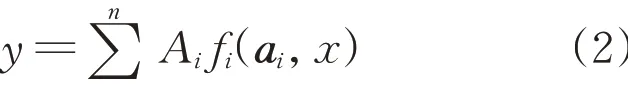
These single-input rule-based models come in the following form[11]

i=1,2,…,c.Here Aiis a fuzzy set defined in the input space while fiis a local function forming the conclusion of the rule.The vector of parameters of the function is ai. The rule-based models are endowed with the inference(mapping)mechanism carried out as follows:
In what follows,with an ultimate intent to eliminate any optimization overhead associated with the design of the rules,we outline a design process which is effortless not calling for any optimization procedures.Consider the data coming in the form of input-output pairs D =(xk,targetk),k=1,2,…,N.
(1)Ais are triangular fuzzy sets with 1/2 overlap between the adjacent membership functions.The modal values of these fuzzy sets are distributed uniformly across the input space.
(2)The conclusion part is a constant function,namely f(x;ai)=yi*where these constants are determined on abasisof thedata.We have
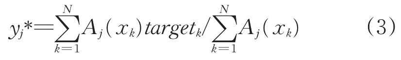
One can easily show that under these assumptions,the input-output mapping of the above rule-based model is nonlinear and realizes a piecewise linear function;refer to Fig.1.
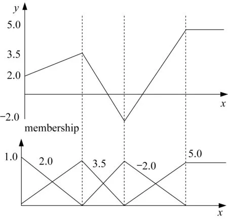
Fig.1 Input-output piecewise-linear characteristics of the fuzzy rule-based model
The nonlinear model(function)produced in this way is fully described by the coordinates of the cutoff points(mj,yj*),j=1,2,…,c.These points are specified by the modal values of the fuzzy sets and the constant conclusions.
Interestingly,the rule-based model can be regarded as a result of multiple linearization of unknown mapping where the linearization is completed around the modal values of the fuzzy sets Ai.Linearization is commonly used in coping with nonlinear problems;the multi-linearization(viz.linearization with several linearization(cut off)points at the same time)arises as an efficient strategy.Not engaging any optimization process(which eliminates any computing overhead),we form therules.
If required,the improvement of the performance of such rule-based model can be achieved in several ways:
(1)Increasing the number of rules which amounts to the increase of the number of the linear segments used to approximate the nonlinear function
(2)Optimizing membership functions of Ai;their location across the unit interval could be optimized
(3)Optimizing constant conclusions of the rules.Here we can determine the constants by solving the following optimization problem:
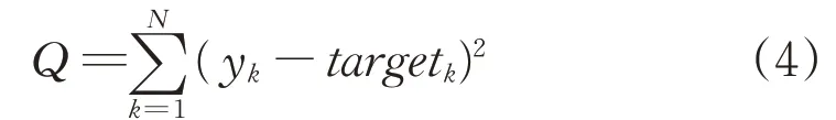
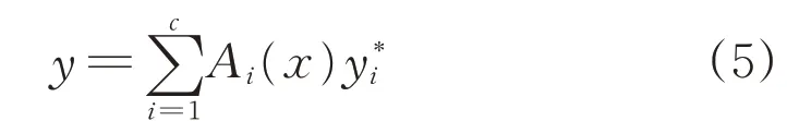
where the minimization is carried out by adjusting the values of y1*,y2*,…,yc*.The result of the model is expressed as
(4)Incorporation of a polynomial format of the functions forming the conclusion parts of the rules.Considering Ais as above,when the conclusion of the rule is a polynomial of order p,the input-output characteristics of the model is a polynomial of order p+1.It is easy to demonstrate this.For any x in the interval[mi,mi+1]there are two rules activated;miand mi+1are the modal values of the corresponding fuzzy sets.This yields the output in the following way y=miPi(x,ai)+mi+1Pi+1(x,ai).Note that miand mi+1are linear functions of x,say mi=b0i+b1ixand mi+1=b0,i+1+b1,i+1x.Therefore y=(b0i+b1ix)·Pi(x,ai)+(b0,i+1+b1,i+1x)Pi+1(x,ai).It is apparent that y is apolynomial of order p+1.
2 Relational characterization of data
The construction of a one-dimensional model does not require any design effort and associated computing overheard.There are some limitations.When dealing only with a single input variable when forming input-output model,we encounter an emerging relational phenomenon of data. This means that for two very closely located inputs,the outputs could vary significantly. In particular,because all but a single variable is considered,one might encounter an extreme situation when for the same input we have two or more different outputs.Note that if the distance between xkand xlbecomes smaller in comparison to the distance between ykand yl,we say the data exhibit a more visible relational character.In limit,if for the same xkand xl(xk=xl)we have ykdifferent from yl,and these data cannot be modeled by a function but a relation.
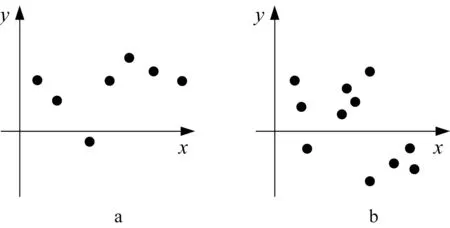
Fig.2 Input-output data and their relational nature
We are interested in the quantification of the degree to which extent the data are of relational nature,viz.
rel=degree(data exhibit relational character)
For instance,intuitively we envision that the data in Fig.2b exhibit more relational character than the one shown in Fig.2a.Having in mind the property of high closeness of two inputs xkand xlassociated with different values(low closeness)of the corresponding outputs ykand yl,we propose the degree of relational nature computed in the following way:
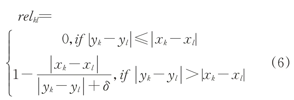
where a small value ofδ,δ>0,prevents from the division by zero.Note that when|xk—xl|becomes lower for the same value of|yk—yl|higher than|xk—xl|,this increases the value of the relationality degree.The global index is determined by taking a sum of relklfor the corresponding pairs of the data,namely
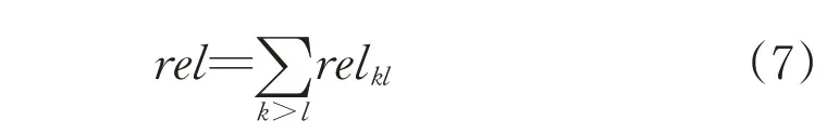
The higher the value of rel,the more evident the relational nature of the one-dimensional data D.
Note that this index exhibits some linkages with the Lipschitz constant K expressing the relationship|yk-yl|<K|xk-xl|.
To illustrate the relational performance of some data,we consider publicly available datasets coming from the Machine Learning Repository https://archive.ics.uci.edu/ml/index.php.For instance,for concrete data,Fig.3 shows the input-output scatter plot for the two variables x5and x8.The more apparent relational nature of x5is also well reflected in the higher values of the index of relationality;a straightforward visual inspection confirms this.The same convincing pattern is conveyed for the two other datasets as well.The same conclusion stems from the analysis of two other datasets(see Fig.4 and Fig.5).
3 Principle of justifiable granularity
The principle of justifiable granularity guides a construction of information granule based on available experimental evidence[7-8].For further extensions and applications,please refer to[4,13,1-14].
In a nutshell,when using this principle,we emphasize that a resulting information granule becomes a summarization of data(viz.the available experimental evidence). The underlying rationale behind the principle is to deliver a concise and abstractcharacterization of the data such that(1)the produced granule is justified in light of the available experimental data,and(2)the granule comes with a well-defined semantics meaning that it can be easily interpreted and becomes distinguishable from the others.
Formally speaking, these two intuitively appealing criteria are expressed by the criterion of coverage and the criterion of specificity.Coverage states how much data are positioned behind the constructed information granule.Put it differently,coverage quantifies an extent to which information granule is supported by available experimental evidence.Specificity,on the other hand,it is concerned with the semantics of information granule stressing the semantics(meaning)of the granule.We focus here on a one-dimensional case of data for which we design information granule.
Coverageand specificity
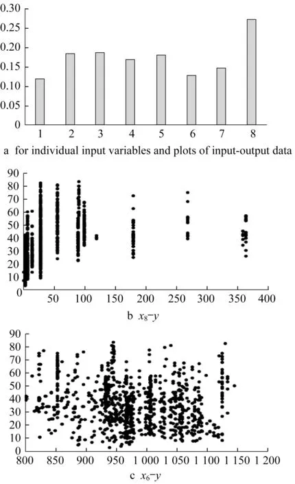
Fig.3 Concrete data:r el
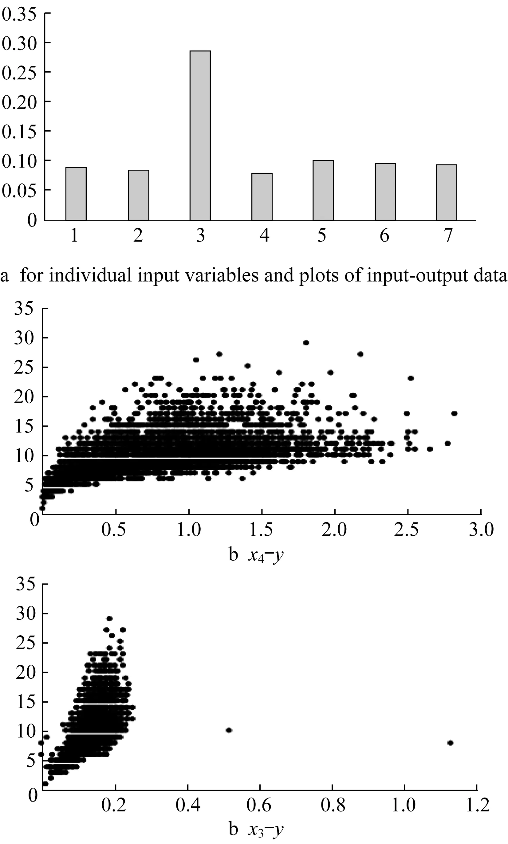
Fig.4 Abalone data:r el
The definition of coverage and specificity requires formalization which depends upon the formal nature of information granule to be formed.As an illustration,consider an interval form of information granule A.In case of intervals built on a basis of onedimensional numeric data(evidence)y1,y2,…,yn,the coverage measure is associated with a count of the number of data embraced by(contained in)A,namely

card(.)denotes the cardinality of A,viz.the number(count)of elements ykbelonging to A.In essence,coverage exhibits a visible probabilistic flavor.Let us recall that the specificity of A,sp(A)is regarded as some decreasing function g of the size(length,in particular)of information granule.If the granule is composed of a single element,sp(A)attains the highest value and returns 1.If A is included in some other information granule B,then sp(A)>sp(B).In a limit case,if A is an entire space of interest sp(A)returns zero.For an intervalvalued information granule A=[a,b],a simple implementation of specificity with g being a linearlydecreasing function comesas
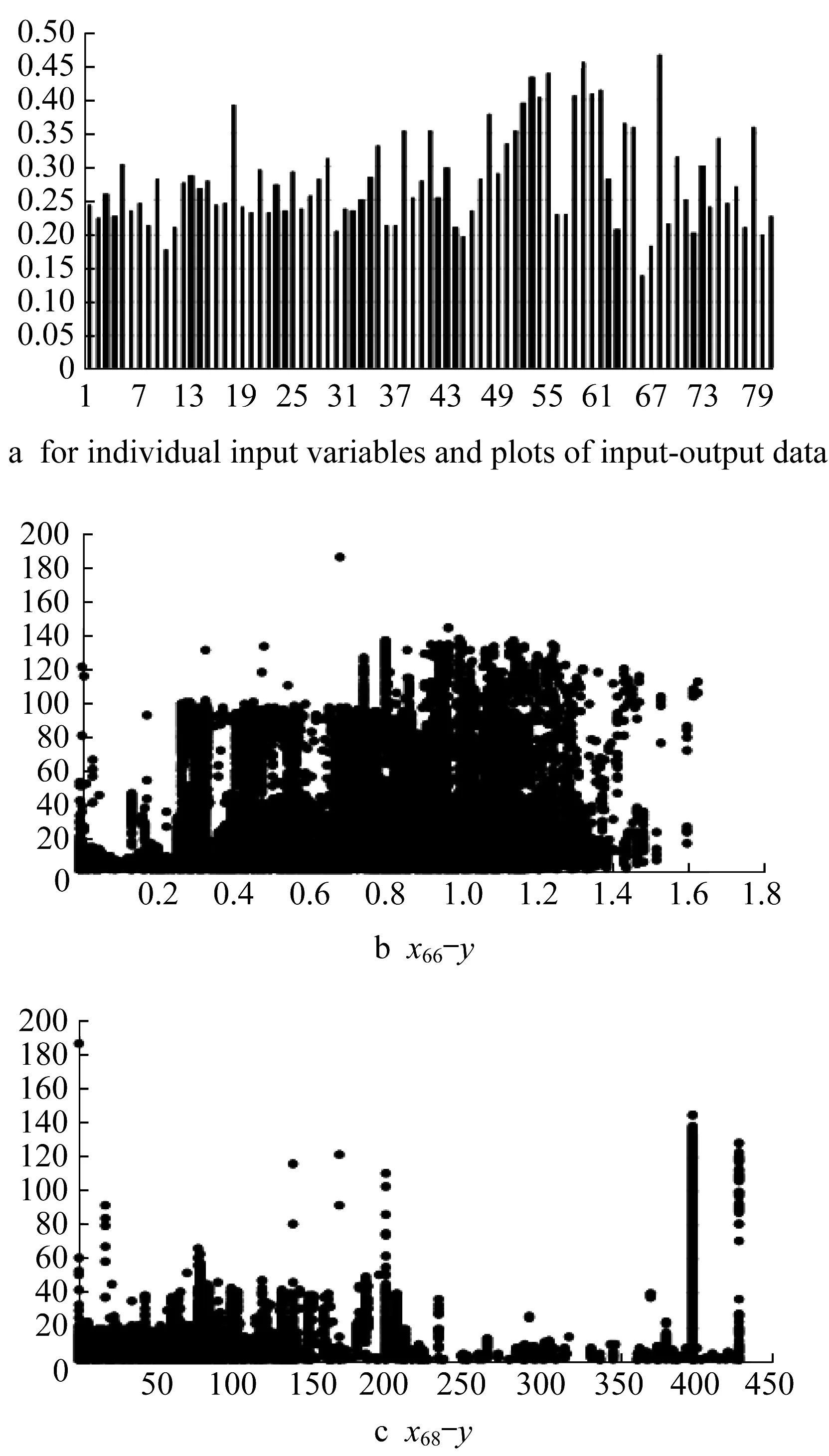
Fig.5 Superconductivity data:r el
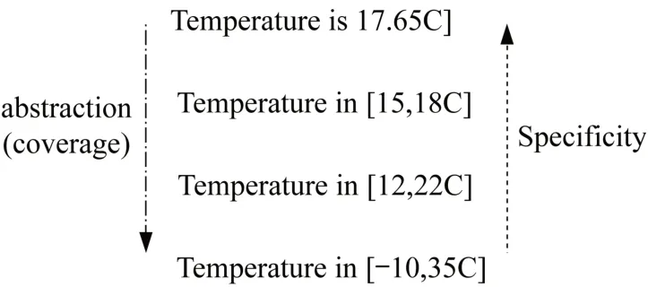
Fig.6 Relationships between abstraction (coverage)and specificity of information granules of temperature

where range stands for an entire space of interest over which intervals(information granules)are defined.
The criteria of coverage and specificity are in an obvious relationship,as shown in Fig.6.We are interested in forecasting temperature:the more specific the statement about this prediction becomes,the lower the likelihood of its satisfaction is.
From the practical perspective,we require that an information granule describing a piece of knowledge has to be meaningful in terms of its existence in light of the experimental evidence and at the same time,it is specific enough.For instance,when making a prediction about temperature,the statement about the predicted temperature 17.65 is highly specific but the likelihood of this prediction being true is practically zero.On the other hand,the piece of knowledge(information granule)describing temperature as an interval[—10,34]lacks specificity (albeit is heavily supported by experimental evidence)and thus its usefulness is highly questionable,as such this information granule is very likely regarded as non-actionable.No doubt,some sound compromise is needed.It is behind the principle of justifiable granularity.
Witnessing the conflicting nature of the two criteria,we introduce the following product of coverage and specificity:

The desired solution(viz. the developed information granule)is the one where the value of V attains its maximum.Formally speaking,consider that an information granule is described by the vector of parameters p,V(p).In case of the interval,p=[a,b].The principle of justifiable granularity applied to experimental evidence returns to an information granulethat maximizes V,popt=argpV(p).
To maximize the index V through the adjusting the parameters of the information granule,two different strategies are encountered
(1)a two-phase development is considered.First a numeric representative(mean,median,modal value,etc.)is determined.It can be sought as an initial representation of the data.Next,the parameters of the information granule are optimized by maximizing V.For instance,in case of an interval[a,b],one has the bounds(a and b)to be determined.These two parameters are determined separately,viz.the values of a and b are determined by maximizing V(a)and V(b).The data used in the maximization of V(b)involves these data larger than the numeric representative. Likewise V(a)is optimized based on the data lower than thisrepresentative.
(2)a single-phase procedure in which all parameters of information granule are determined at the same time.Here a numeric representative is not required.
The two-phase algorithm works as follows.Having a certain numeric representative of X,say the mean,it can be regarded as a rough initial representative of the data.In the second phase,we separately determine the lower bound(a)and the upper bound(b)of the interval by maximizing the product of the coverage and specificity as formulated by the optimization criterion.This simplifies the process of building the granule as we encounter two separateoptimization tasks
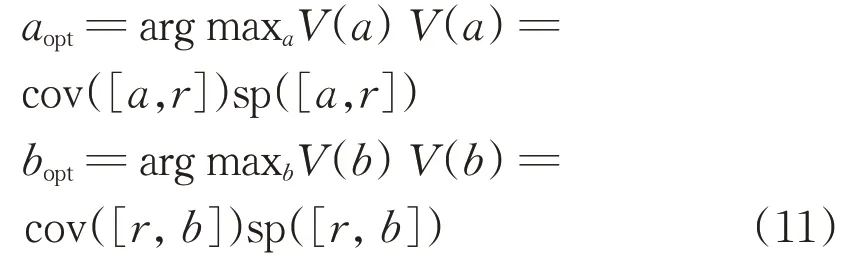
We calculate cov([r,b])=card{yk|yk∈[r,b]}/n.The specificity model has to be provided in advance.Its simplest linear version is expressed as sp([r,b])=1—|b—r|/(ymax—r).By sweeping through possible values of b positioned within the range[r,ymax],we observe that the coverage is a stair-wise increasing function whereas the specificity decreases linearly,(see Fig.7).The maximum of theproduct can beeasily determined.
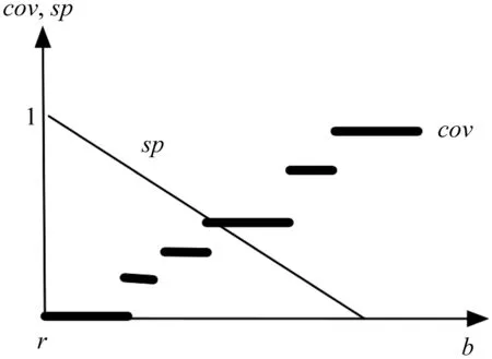
Fig.7 Example plots of coverage and specificity(linear model)regarded as a function of b
The determination of the optimal value of the lower bound of the interval a is completed in the same way as above.We determine the coverage by counting the data located to the left from the numeric representative r,namely cov([a,r])=card{yk|yk∈[a,r]}/n and compute the specificity as sp([a,r])=1—|a—r|/(r—ymin).
The algorithmic essence of the principle is captured in Fig.8 where we emphasize the two design phases,namely the determination of the numeric representative(aggregation)followed by the optimization of the criterion V which is realized independently for the bounds a and b.
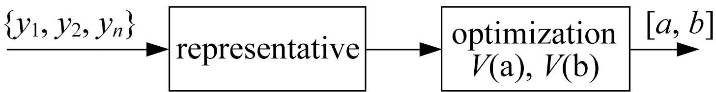
Fig.8 Two step-design of interval information granule
As a way of constructing information granules,the principle of justifiable granularity exhibits a significant level of generality in two essential ways.First,given the underlying requirements of coverage and specificity,different formalisms of information granules can be engaged. Second,experimental evidence could be expressed as information granules articulated in different formalisms based on which certain information granule isbeing formed.
The principle of justifiable granularity highlights an important facet of elevation of the type of information granularity:the result of capturing a number of pieces of numeric experimental evidence comes as a single abstract entity—information granule.As various numeric data can be thought as information granule of type-0,the result becomes a single information granule of type-1.This is a general phenomenon of elevation of the type of information granularity.The increased level of abstraction is a direct consequence of the diversity present in the originally available granules.This elevation effect is of a general nature and can be emphasized by stating that when dealing with experimental evidence composed of a set of information granules of type-n,the result becomes a single information granule of type(n+1).
4 Augmentation of the principle of justifiable granularity:error profiles
The principle of justifiable granularity can be further extended by introducing a so-called error profile.
The coverage criterion conveyed by Eq.(8)reflects how information granule covers the data.Quite often in modeling environment one obtains information granule whose quality has to be evaluated vis-à-vis error viz the difference between the numeric result of the model and the numeric experimental data expressed as ek=targetk—ykwhere ykis the k-th result produced by the model. Obviously,we anticipate that a sound model should produce values of error close to zero however a notion of close to zero requires more elaboration.Here a concept of error profile comes into the picture.
The error profile f(e)is an information granule(typically,a fuzzy set)whose membership function describes in detail to which extent the error is acceptable.Some examples of the profiles are shown in Fig.9.Their flexibility helps cope with the particular requirements of modeling.For instance,Fig.9a the profile is binary.We do not tolerate any error beyond the bounds—emax,emax.There could be some membership functions facilitating a smooth transition from full acceptance to a complete lack of acceptance.The shapes of the membership functions could vary being symmetric or points at higher acceptance in the presence of values of error close to zero and then dropping more visibly.Figure 9c illustrates the piecewise character where more flexibility is accommodated.Notably,the profiles need not to be symmetric.
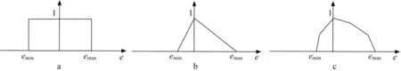
Fig.9 Examples of error profiles f(e)
The error profile is made a part of computing concerning the coverage criterion,namely in calculationsof b one has
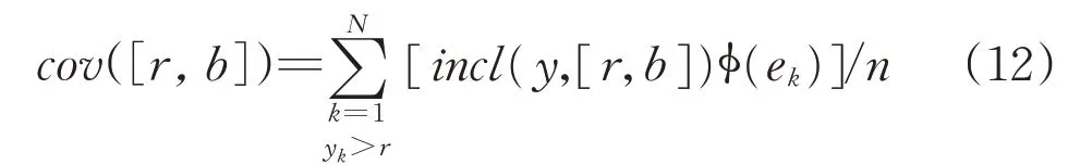
where incl(x,[a,b])is a Boolean predicate such that it returns 1 if x is included(covered)in the interval and 0 otherwise. The computing of specificity iscarried out as before.
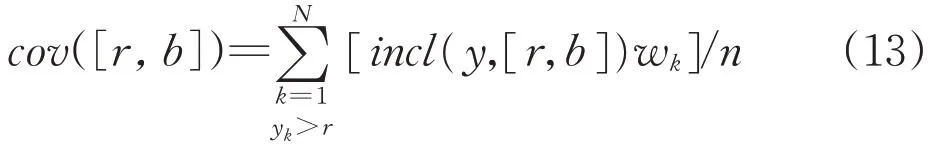
The principle can also involve weights and in this situation,they are a part of the coverage criterion.The values of the weights are determined based on the performance of the individual local models.Given that their performance is described by the index Q1,Q2,…,Qn(those could be the results of computing the RMSE value produced for each model),the weight can be made a decreasing function of the Qk,say wk=exp(—(Qk—Qmin)/(Qmax—Qmin)with Qminand Qmaxbeing the values of Q for the best and the words model.
The coverage expression comes in the form of
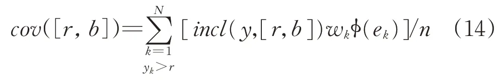
The accommodation of both the weights and the error profile gives rise to the following expression:
5 Aggregation operators
The data y1,y2,…,ynare to aggregated(fused).Formally,an aggregation operation agg:[0,1]n→[0,1]is an n-argument mapping satisfying the following requirements:
(1)Boundary condition agg(0,0,…0)=0,agg(1,1,…,1)=1
(2)Monotonicity agg(y1,y2,…,yn)≥
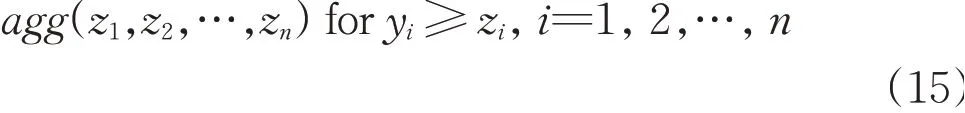
Triangular norms and conforms[5-6,10,12]are examples of aggregation operations.However there are a number of other interesting alternatives.The averaging operator deserves attention as it offers a great deal of flexibility. An averaging operator(generalized mean)is expressed in the following parameterized form[1]:
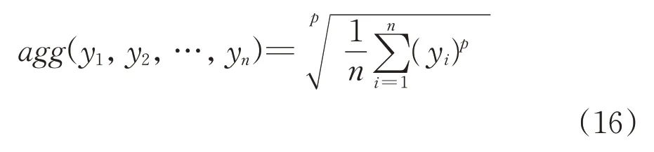
When p is a certain parameter,the class of generalized mean is made a generalized class of operators.The averaging operator is idempotent,commutative,monotonic and satisfies the boundary conditions agg(0,0,…,0)=0,agg(1,1,…,1)=1.
Depending on the values of the parameter p,there are several interesting cases
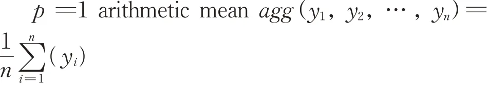
p→0 geometric mean agg(y1,y2,…,yn)=(y1y2…yn)1/n
p=—1 harmonic mean agg(y1,y2,…,
p→-∞maximum agg(y1,y2,…,yn)=max(y1,y2,…,yn)
p→→∞minimum agg(y1,y2,…,yn)=min(y1,y2,…,yn)
6 Overall architecture of granular aggregation of multiview models
The overall architecture of the global model is shown in Fig.10.
Here we encounter n one-dimensional rule-based models M1,M2,…,Mnfollowed by the aggregation module where the results are aggregated.In contrast to commonly studied methods of aggregation,an important point is that the aggregation of numeric results gives rise to an information granule.The granularity of the results is crucial to the evaluation of the quality of the overall architecture.Again,here we look at the coverage and specificity criteria as means to evaluate the obtained result.
In more detail,let us consider that the models were constructed based on the input-output data(xk,targetk)where xkis an n-dimensional vector of inputs,k=1,2,…,N.The model Miis constructed by taking the i-th coordinate of the input data,viz(xki,targetk).The coverageis expressed as:


Fig.10 Granular aggregation of multiview models
while the specificity is given in the form of
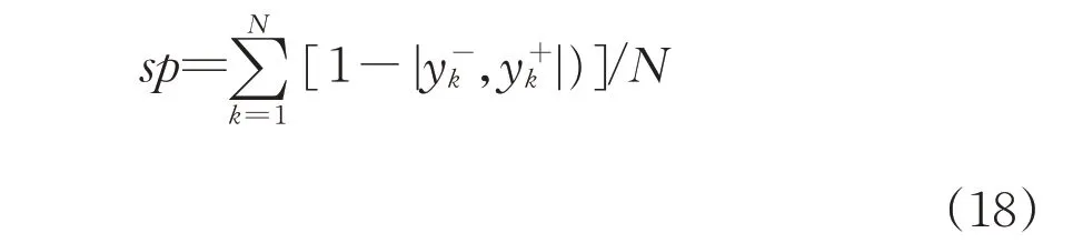
The quality of the architecture is expressed as the product of these two criteria;cov*sp the higher the product,the better the quality becomes.
7 Granular one-dimensional rulebased models and their granular aggregation
The one-dimensional models are not ideal(especially because of the relational format of the data).We augment the numeric output of the model by its granular extension by admitting that it comes as an interval of some level of information granularity e spread around the numeric result produced by the rulebased model.Information granularity is reflective of the diversity of the results.
Let us refer to the piecewise linear characteristics of the model,(see Fig.11).
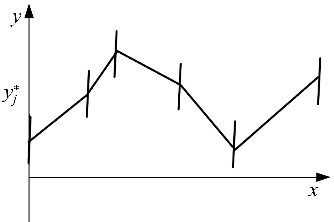
Fig.11 Piecewise relationships with interval-valued cutoff points
Recall that the input-output relationship is fully described by the cutoff points(mj,yj*).We quantify the quality of the model by admitting a certain level of information granularity e assuming values in the unit interval and yielding a granular(interval-valued)outputs.The numeric values are made granular by admitting the level e.The following alternative is sought:
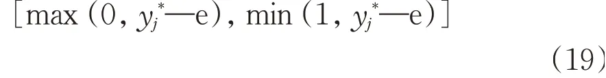
This yields the granular outputYfor givenx
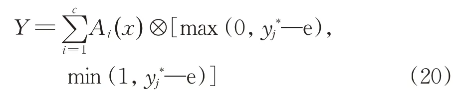
⊗stands for the interval multiplication.This gives rise to the following interval Y=[y-,y+]where(x)max(0,yi*—e)and y+=(x)min(1,yi*+e).
For any xkin the data set,we determine the corresponding Ykand next compute coverage and specificity,V=cov*sp.Evidently V is a function of e so its value has to be optimized by searching for the maximal value of V,eopt=arg maxeV(e).
Progressing in this way with all the onedimensional models we obtain associated optimal levels of information granularity,e1,e2,…,en.As a result,for any x,these models return Y1,Y2,..Yn.This gives rise to the augmented architecture illustrated in Fig.12.
Noticeable is a fact that the arguments entering the aggregation process are information granules themselves.This implies,in light of the principle of allocation of information granularity,the result becomes an information granule of higher type than the arguments being aggregated,viz.in this case socalled granular intervals.They are intervals whose bounds are information granules themselves.One can denote the granular interval as Y~=[[y--,y-+],[y+-,y++]]where y-+<y+-.
The detailed calculations concerning the granular bounds of the information granule are carried out by engaging lower bounds of Y1,Y2,…,Yn.Likewise the computing of the upper bound of Y~involves the use of the upper bounds of Y1,Y2,…,Yn.In this construction one has to make sure that the constraint issatisfied.
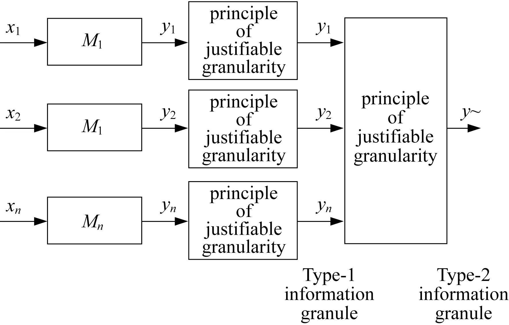
Fig.12 Augmented architecture of the model:note elevation of type of information granularity when progressing towards consecutive phases of aggregation
8 Conclusions
In his paper,we formulated and delivered a solution to the problem of granular aggregation of multiview models and identified a sound argument behind the emergence of the problem. It is demonstrated that a highly dimensional problem can fit well the developed framework. It has been advocated that the aggregation mechanism producing information granules helps quantify the quality of fusion and reflect upon the diversity present among the results produced by the individual models.The principle of justifiable granularity becomes instrumental in constructing information granules.It is also shown that the elevation of the type of information granularity(to type-1 or type-2)becomes reflective of the increased level of abstraction ofmodeling.
There are several directions worth pursuing as long-term objectives. While in this study,for illustrative purposes,we engage interval calculus to realize the discussed architecture,other alternatives of formal frameworks,say fuzzy sets and rough sets,are to be discussed.The general architecture remains the same;however,some interesting conceptual and computing insights could be gained in this way.Architecturally,we studied a two-level topology:a collection of one-dimensional rule-based models followed by an aggregation module.An interesting alternative could be to investigate low-dimensional rules(with two or three conditions,which is still feasible)and ensuing hierarchical structures along with agranular quantification of the model.
猜你喜欢
无机化学学报(2022年10期)2022-10-10
物流技术与应用(2022年5期)2022-06-17
同济大学学报(自然科学版)(2022年4期)2022-05-13
华夏教师(2021年28期)2021-05-23
华夏教师(2021年28期)2021-05-23
黄埔(2020年4期)2020-08-13
黄埔(2020年4期)2020-08-13
意林·作文素材(2018年7期)2018-05-30
作文周刊·高一版(2016年30期)2017-03-03
人生十六七(2016年27期)2016-02-18
