一维函数方法求解原子和分子薛定谔方程

SARWONO Yanoar Pribadi，UR RAHMAN Faiz，赵润东，张瑞勤

（1.香港城市大学物理系,香港；2.北京计算科学研究中心,北京100193；3.北京航空航天大学物理学院,北京100191；4.深圳京鲁计算科学应用研究院,深圳518131）

1 Introduction

Birkhoff［1］and Young［2］suggested that to obtain approximate solutions to the Schrödinger differential equation with a rigorously numerical technique would be both interesting and desirable.This paper presents the theory and procedure for the application of the one-dimensional functions to the atomic and molecular calculations.One-dimensional hydrogen atom（1D H function），for example，has found many applications in high magnetic fields［3］，semiconductor quantum wires［4］，carbon nanotubes［5］，and polymers［6］.Nonetheless，the application of the 1D H functions to atomic and molecular calculations has not yet much investigated.Unlike Gaussian type orbitals（GTO）［7—10］which use the analytical and the recursive integration scheme of the twoelectron integrals calculation or Slater type orbitals（STO）［11，12］which have an extensive analytical energy expressions table［13］as well as basis size efficient，analytical evaluation of energy terms does not exist once the 1D functions such as the 1D H functions are employed.Hence，numerical methods must be applied.The 1D functions are regarded as more general basis functions since the 1D functions can generally repeat the result of the corresponding 3D counterparts but not otherwise，as in the Gaussian orbitals wheree-r2is the product of three 1D Gaussians inx，y，andzcoordinates［14］for the radial distancer= ( )x2+y2+z2.Unlike the standard basis functions，the 1D functions use Cartesian coordinates as a reference frame where common numerical methods of partial-differential equations are formulated so the iteration matrix can be simplified.The normalizability of theNdimensional wavefunction expanded with the 1D functions is satisfied by performing theNproduct of the 1D functions in each dimension like the particle in a box problem.Therefore，the 1D function approach is unique in two aspects.First，the approach is purely numerical methods to solve the Schrödinger equation.Second，the approach is completely the first application of the 1D functions in atomic and molecular calculations.

Another compelling reason to develop the 1D function approach is the difficulties of the standard electronic structure methods to treat electronic correlation；hence，an efficient many-body approach is required to deal with the many-body systems with accurate treatment of electron correlations.In the conventional selfconsistent field（SCF）calculations such as density functional theory（DFT）［15，16］and Hartree-Fock（HF）［17，18］，the many-electron problems are proceeded with separating them into a set of accessible single-electron selfconsistent eigenvalue equations.Therefore，HF neglects the many-body effects of electron correlation，while DFT includes exchange-correlation functional to account for the effects［19—21］.These separations of particles approaches are different in nature from the non-SCF accurate variational calculations of molecular（atomic）energy levels such as the James-Coolidge calculations［22，23］（Hylleraas calculations and the hypersherical coordinates methods［24—32］）for the H2molecule（the helium atom and its isoelectronic ions）.The corresponding accurate variational calculations have tackled the Schrödinger equations in their full dimensionality and as full many-electron problems.To solve the time-independent Schrödinger equation of the many-electron atomic and molecular problems which in the present work we limit ourselves to two-electron cases，the employed 1D function approach follows neither the SCF techniques nor the accurate approaches.The 1D function approach assumes the separability ansatz of the many-electron by the Cartesian components，rather than by particle，as stated in recent papers［33—37］.

The primary significance of the 1D function approach over any such particle-separability approaches is to treat exactly the electron correlation.The approach can include many-body effects directly；hence，electron correlation is more accurately treated，as we shall demonstrate when the repulsion energy comparison is performed.Another key advantage is that the basis can be expanded in all Hilbert space directions at once.In the present work，we use real-space grids representation of the Hamiltonian and the wavefunction.The former is represented as sparse matrices and the latter as vectors.This brings to the next benefit which allows iterative methods of residual vector correction［33，34，36，37］to be implemented.Iterations that repeatedly apply the Hamiltonian operatoron a wavefunctionare conveniently carried out since the action of an operator on a wavefunction is implemented numerically as a straightforward matrix-vector product.Unlike the plane wave basis［35］integral evaluations which require additional steps such as the Fourier transform，the numerical integrals are easily performed in the real-space 1D functions basis with the row-vector matrix column-vector product times the power of dimensions of the grid spacing size as the scheme.This feature is particularly useful when dealing with the multicenter integral problem［38，39］present in molecular calculations.Unlike the previous partitioning scheme which divides an integral over the entire molecular volume into a sum of atomic orbitals［40］，the 1D function approach does not require such schemes.The residual norm is progressively made small until convergence is reached.Hence，our approach is similar to the previous accurate variational calculations for helium and its isoelectronic ions and hydrogen molecules where SCF is not needed.Furthermore，the behavior of numerical convergence is known.

In the present work，we present the applications of the 1D function approach to obtain the ground state of the hydrogen atom and the helium atom and their isoelectronic ions and the hydrogen molecule and its ions.The 1D function approach is preferably very general since the only approximations included are the change of a differential equation with a set of finite-difference equations.The resulting error in this approximation can be reduced to suitably small.However，in practice the approach is restricted by computer memory size and computer time cost.Like common perturbation and variational techniques which give accurate results for manyelectron problems provided the number of terms is large so that the correlation effects are properly treated，the present method can describe correlation properly if the grid spacing size is sufficiently small.Hence，any numerical error is understandable from the finite-difference approximation and the results can be straightforwardly compared with the experimental ones.In terms of many-electron problems，if the 1D function approach can reach to four-electrons calculations，large electronic structure problem can be considered as solvedviaa corresponding contracted Schrodinger equation［41］.

2 Theory

2.1 Vectors and Functions

In three-dimensional（3D）space，vectors r characterize points and are denoted with the 3-tuple

On this space，scalar function is usually expressed asφ，

In a separable solution，the scalar function can be written as the product of its spatial components

where the functionsX，Y，andZare in 1D.Such problems are not considered in the 1D function approach，rather the nonseparable ones are studied.An example of a nonseparable problem is the Coulombic potential between charges at a distance

Represented with the 3-tuple Cartesian components，no existence of the product functionφ（x，y，z）equal to the Coulombic potentialV(r).A closer approximation to the Coulombic potential is foundviaa sum of separable-like functions［42，43］.

2.2 Optimally Separable Hamiltonian

In atomic units，the Hamiltonian of a system ofNelectrons andKnuclei with chargesZwithin Born-Oppenheimer approximations is

where the first term is the kinetic energy of theith electron，the second term is the electron-electron interaction energy term，the third term is the ionic energy interaction betweenith electron andlth nucleus located at Rl，and the last term is the nuclei repulsion term.The indexiandjrefer to the electrons andl，l′to the nuclei.TheN-electron wavefunctionψ(r1，r2，…，rN)satisfies the Schrödinger equation

whereEis the energy of the system.

Our 1D approach does not necessitate any coordinate transformation from the original Schrödinger equation formulated in the Cartesian coordinate.Because of the rapid increase of the dimensional size，few-electron problem is suitable for this approach.For a one-electron system found in the hydrogen atom and its isoelectronic series or in the hydrogen molecular ion，a wavefunction constructed by 1D functions has the general form of

whereφ(x)is an eigenfunction of some 2D single-component one-electron effective HamiltonianSuch basis forms an optimally separable approximate Hamiltonian

whereφ(x1，x2)is an eigenfunction of some 4D single-component two-electron effective HamiltonianSimilarly，such basis will form an optimally separable approximate Hamiltoniantogether with the 2D single-component two-electron identity operator

In terms of the 1D single-component one-electron identity operatorand the 2D single-component oneelectron effective Hamiltonianthe optimally separable Hamiltonian for a two-electron system of 6D is written as

2.3 One-dimensional Functions as the Basis

The types of 1D functions to be considered generally fall into two categories.First is the one that is the solution of the corresponding 1D equation［44—50］，exemplified in the case of the 1D hydrogen（1D H）function which is a symmetric and square-integrable function with the cusp at origin.The expression of the 1D functions in this category is generally very intricate like the composite of the products of more than one simple functions.In practice，the functions are conveniently found through a numerical method.The second category is the one which is the 1D version of the corresponding 3D functions counterpart，such as 1D Gaussian and 1D Slater.Their expressions are simpler than the first category with their properties resembling their 3D functions like the origin-centered 1D Gaussian［51—53］or the cusp possessed in the 1D Slater［54—57］.This serves their purposes for convenient integration.In the present work，the 1D H function is implemented to obtain the solution of the hydrogen atom［33］.Subsequently，a two-dimensional single-component two-electron of helium and its isoelectronic ions wavefunction is applied to the helium and its isoelectronic ions calculations［33，34，37］.Similarly，the ground state of a molecule can be constructed from its single component［36］.

The expression of the 1D H［47］function is given as

whereAis the normalization constant，nis the principal quantum number，andis the generalized Laguerre polynomial，andkcorresponds to the 1D H energyEasThe trial solutions for the hydrogenic atoms are then constructed from their single component as

wherecijkare constants andNis the number of the grid points in one-dimension.In this basis，the optimally separable Hamiltonianis represented.As the trial wavefunction Eq.（13）is the eigenstate of thethe eigenvalueE(0)is less superior than the ground state energy of the hydrogenic system.Next，we choose a 2D single-component two-electron of helium and its isoelectronic ions wavefunctionφ(x1，x2)as the basis set for the helium and its isoelectronic ions calculations.The 2D wavefunctionφ(x1，x2)is the solution of the corresponding 2D He Schrödinger wave equation

where the first two terms are the kinetic energy terms in each dimensions，the third and the fourth terms are the electron interaction terms with a nucleus at the center，and the last term is the electron-electron interaction term，andζis the corresponding energy eigenvalue of the 2D He.The constantβ=0.00001 has been added to avoid the infinite solution atxi=0，i=1，2［50］.In the grid representation(x1i，y1j，z1k，x2l，y2m，z2n)，the trial wavefunction is written as

whereNis the number of grid points of 1D functions in one component andcijklmnis the coefficients of expansion.Thus for two-electron generalization，the basis size grows asN6.

Like the atomic case，a trial variation function to describe the ground state of a molecule can be constructed from its 1D components.For example，thetrial variation functionψ(0)(r)can be constructed from its 1D componentsφ(x)with coefficients

whereφ(x)satisfies the corresponding 1D Schrodinger equation of

for two nuclei atxaandxbwith the 1D energy in one componentεx.For a two-electron molecule such as H2，the trial variation function can be expanded with the product of its 2D two-electron componentsφ(x1，x2)

The basis functionφ(x1，x2)is obtained from the 2D Schrödinger equation version of H2

2.4 Space Discretization and Multidimensional Numerical Integration

To represent theN-electron Hamiltonian Eq.（6），uniform orthogonal 3N-dimensional grids of equal spacing sizehneed to be generated.Each side of the uniform 3N-D hypercubic grids is of length 2r0.The uniform real-space grids allow for a simple discretization of the Schrödinger equation so that physical quantities like wavefunctions and potentials are numerically represented by the values at the grid points.The maximum range of each position coordinater0is related with the grid spacing sizehand the number of the grid pointsThe number of the grid pointsNis determined up to computational resources，while the optimum grid spacing sizehis chosen to minimize energy.Derivatives are calculated with finite-differences where in the present work the standard-order is implemented.The Laplacian is the sum of the second-order derivative in each dimension.Therefore，for a two-electron case，six second-order derivatives are constructed.Hence，the accuracy of the discretization is determined by the grid spacing size and the finite-difference order used for the derivatives.The potential energy operators are represented as diagonal matrices as a consequence of a certain quadrature approximation［58］.The Coulombic singularity is avoided by setting even number of grid pointsN.The electron repulsion is handled by restricting the two electrons not to occupy the same space.

Having put all quantities in the real-space grid representations where the operators are represented as matrices and the wavefunctions as vectors，one can perform the convenient multidimensional numerical integration over the Cartesian grids where the accuracy of the scheme largely depends on the number of grid points and the grid spacing size.The action of the operator on the wavefunction is simply a straightforward matrixvector product.In the case of the H2matrix elements calculations，the integrals of the HamiltonianH(r1，r2)over 6D space transform into sum over grid pointsm，nof grid spacing sizehin the grid points positions rm，rn

The multidimensional integral scheme above clearly provides a convenient alternative route to evaluate any integrals present in the atomic and molecular calculations beside the analytical product theorem formulation of the Gaussian type orbitals or the extensive tables of Slater type orbitals.Unlike the plane wave basis，the integrals evaluation of the 1D functions does not require reciprocal space or Fast Fourier transform library.

2.5 Residual Vector Correction

For ground state calculation，the residual vector correction which is based on iterative Krylov subspace methods of orderO(N2)is more suitable than the conventional diagonalization of orderO(N3).The reason is that the Hamiltonian operators are large sparse matrices in the real-space grid representation.Therefore，the computational cost of exact diagonalization scheme becomes very expensive.On the other hand，the sparsity of the matrices causes the iterative diagonalization which involves the matrix-vector multiplication more appealing.The central quantity in the iterative method is the residual function.In the two-electron case atmiteration，the residual functionobtained from the trial wavefunctionand its energyE（m）is in the form of

The definition of the residual above allows the search to be performed in the direction of the greatest decrease，unlike the preconditioned residual as a consequence of the perturbation theory［59，60］.A new and refined wavefunctionψ(m+1)（r1，r2）is given as

which is the linear combination of the residual functionand the current resultThe expansion coefficientsC0andC1provide the necessary step of the search to minimize the energy withC0approaching unity andC1becoming increasingly small.They can be determined from another smaller 2×2 generalized eigenvalue problem in themstep

where in the iterative subspace the Hamiltonian matrixHij，the overlap matrixthe optimized energyE，and the trial stepsCj，j=0，m.The iteration is terminated once the difference between the consecutive energiesEin Eq.（23）achieves 0.0003 eV.

3 Results and Discussion

3.1 Hydrogen Atom and Its Isoelectronic Ions from 1D H Function

To test the approach，a single-electron calculation of the hydrogen atom and its isoelectronic ions ground electronic state are performed.The exact ground state energy of the H，He+，Li2+，Be3+are known analytically to be-13.6057，-54.4228，-122.4513 and-217.6912 eV，respectively［61］.The results of the 1D function approach can then be straightforwardly assessed in terms of accuracy and convergence.In the hydrogenic cases although only one electron is present and no electron correlation effect，the test is still important，particularly to demonstrate how the Coulomb singularity in the potential energy is to be handled.One can adjust the number of grid points so that none of the grid points lies directly on the nucleus.

Once the Hamiltonian is represented with the finite-difference method，the residual vector correction Eqs.（21），（22），and（23）is implemented to perform the necessary refinements to obtain more accurate wavefunction.The plot of the coefficientsC0andC1are shown in Fig.S1（see the Supporting Information of this paper）.The negative ratio ofC0/C1shows the correct steepest descent search direction where the negative gradient of the Rayleigh quotient is used.TheC0value that is closer to one ensures the correction occurs along the residual vector and the orthonormality with the previous search direction is maintained.The positive coefficientC1means that the gradient of the Rayleigh quotient being in the same direction as the residual unlike the linear system case.The gradient vector trial step is large in the several first iterations.The size ofC1is largely affected by the implemented number of grid pointsNand the grid spacing sizeh，which is understood becauseNdetermines the matrix size of the Hamiltonian whilehaffects the location of the ground state energy through the numerical integration scheme.Correspondingly，the search performed byC1goes to the correct ground state and prevents from moving to the wrong state.Near the convergence pointC1shows a see-saw nature until convergence，showing the stability of the residual vector correction.

The Rayleigh-quotient minimization performed with the residual vector correction has straightforward effect on the iterated energy and the virial ratio shown in Fig.S2（see the Supporting Information of this paper）.In the variational process to obtain a converged energy，the iterated energy is corrected starting from the upper bound until convergence［62］.As the energy is refined，the virial ratio shows improvement to be closer to the exact value of two.

For the shortest grid spacing sizehwhich has the largest number of grid points per dimensionN，the ground state energy of the hydrogen and its isoelectronic ions are converged to a 0.0027 meV or even better（Table 1）.This one-electron calculation is a proof of concept that the 0.0027 meV or better accuracy is reachable with the 1D function approach.As seen，the error increases for largerZ.This stems from the fact that in all calculations the number of grid points per Cartesian dimensionNused isN=400 despite heavier nuclei require finer grid spacing size to account for their Coulomb attraction potential and their kinetic energy shown in Table S1（see the Supporting Information of this paper）.The kinetic energy and the ionic energy error show the tendency to have increasing error for largerZ，nonetheless the virial ratio remains in the accuracy of 2.0 in the present calculations.The improvement can be proceeded with a technique to evaluate the ionic energy more accurately without requiring too finer grid spacing size known as electron centers displacement［37］which will be demonstrated in the helium atom and its isoelectronic ions calculations part.The Coulombic singularity of the nuclear attraction can also be better treated with the use of various approximations such as“softened”Coulomb potentials［63］，reduced dimensionality of physical space［64］，approximate 3D discrete variable representation potentials［65，66］，or the use of the logarithmic grids［14，67，68］followed with the necessary coordinate transformation of the equation.The kinetic energy may be improved using either higher order second order derivative finite-difference method［69］or analytical form of discrete variable representation kinetic energy matrix［70，71］.

Table 1 Ground state energy of the hydrogen atom and isoelectronic series obtained with the 1D function approach and the exact value a

If one plots the error relative to the exact energy as a function of the grid spacing sizehas shown in Fig.S3（see the Supporting Information of this paper），a simple quadratic equation can be obtained.This is seen from the value ofR2which is nearly equal to one.The quadratic scaling is anticipated because of the Coulombic singularity，the choice of the Cartesian 1D H basis，and the finite-difference approximation.Such scaling shows that the convergence is fast in the region far from the accurate but slow close to the accurate value.From Fig.S3 the required grid spacing size to reproduce error free relative to exact energy can be calculated from finding the root of the quadratic equation.The roots confirm that finer grid spacing size is required to describe energy more accurately for atoms with an increasingZ.

In the following，the wavefunction analysis is given.First，the obtained wavefunction can be surfaceplotted against thexandycoordinate，displaying a cusp，a characteristic of 1s，shown in the inset of Fig.S4（A）（see the Supporting Information of this paper）.The cusp can be reproduced and the vanishing wavefunction far from nucleus is seen.Second，as seen from Fig.S4（A）the obtained wavefunctions coincide with the exact wavefunctions when plotted against the radial distance.The ion Be3+has the steepest slope and results in the highest cusp than that of other species with lowerZ.The phenomenon is related to the kinetic and the potential energy to conserve the Heisenberg uncertainty principle.Third，Fig.S4（B）shows the radial distribution function of the hydrogen atom and its isoelectronic ions.A single peak of 1scharacteristic is observed.For heavier atoms/ions，the peaks are closer to the nucleus than those of lowerZ.

3.2 Helium Atom and Its Isoelectronic Ions from 2D He Function

The developments of the coefficientsC0andC1are shown in Fig.S5（see the Supporting Information of this paper）.Overall，the performance of the optimization is the same as that implemented in the hydrogenic cases.The coefficientC0progresses toward one with the opposite sign compared with the coefficientC1，indicating the search occurs in the steepest descent and in the same direction as the negative of the Rayleigh quotient gradient.The magnitude ofC0in the helium optimization is about three times larger than that in the hydrogen cases，corresponding to the larger grid spacing size implemented in the helium case due to the fast-growing scale of the required basis functions.The grid spacing size affects the evaluation of the Rayleigh quotient in the minimization process through the implemented numerical integration scheme which depends onC1.As the Rayleigh quotient minimization is a variational process，the iterative energy of the helium approaches the true energy variationally.Consequently，the virial ratio-V/Tmoves closer to the exact value of 2 which is depicted in Fig.S6（see the Supporting Information of this paper）.

The repulsion energy convergence of the helium atom and its isoelectronic ions where the number of grid points per dimensionN=30 and where the electron centers displacement technique has been implemented［37］are shown in Table 2.The repulsion energy where the non-classical effect is present possesses error within 1.3606 eV or better.In all calculated atomic systems，the calculated repulsion energies are more accurate than the HF results［72］which can reach 2.7211 eV in error.The reason is that the pair-wise electron approach of the 1D function approach treats directly and exactly the electron-electron interaction.If considerably finer grid spacing size and more number of grid points are applied，one will obtain the accurate result for the integration scheme for the repulsion energy.

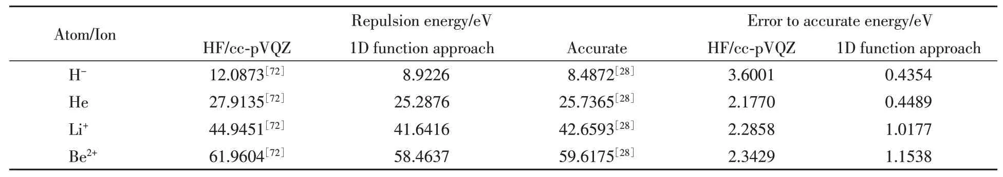
Table 2 Electron-electron effect present in the repulsion energy of the total energy component of the helium atom and its isoelectronic ions

If one plots the error relative to the accurate resultsversusthe grid spacing size，a simple relation will be found from which the required grid spacing size to reproduce error free relative to accurate energy can be obtained［37］.In contrast to the hydrogen and its isoelectronic case，the helium case shows a power scaling with the power less than 2.This situation is understandable since the energy of the helium is obtained with larger grid spacing size than that of the hydrogen atom and causes the behavior of the error in the finite-difference method has not reached quadratic scaling.The two-electron wavefunction of the helium atom and its isoelectronic series allow for single-electron functions plot such as single-electron wavefunction，densities，and radial distribution.Fig.1 shows the ground state radial distribution function obtained with the HF，the DFT，and the 1D function approach.Compared with the single-electron methods，the electron correlation effect is seen in the decrease of the probability to find an electron at radial distance between 0.4 and 1.5 bohr［73］.

Fig.1 Radial distribution function obtained with the 1D function approach compared with that obtained with the DFT method and the HF method

The scaled radial distribution function for the ground state of the helium atom and its isoelectronic ions are given in Fig.S7（see the Supporting Information of this paper）.Consistent with the 1s1scharacter of the ground state，a single peak is observed.Fig.S7 also shows that for heavier atoms the peaks are closer to the nucleus.

3.3 Hydrogen Molecule and Ions from 1D H Function

The performance and the behavior of the implemented residual vector correction to obtain the ground state and the bond length of molecule are the same as those in the atomic case.The coefficientC0trend toward unity after several number of iterations is observed.CoefficientC1is progressively small and shows“see-saw”pattern.The search occurs in the gradient descent direction whereC0andC1have opposite sign.The magnitude ofC1is influenced by the implemented grid spacing size so thatC1is larger in the H2case than in the H+2case.Inherent in the implemented residual vector correction，the true energy is achieved variationally that is from rigid upper bound to the converged value.

As seen in Table 3，the present grid specification leads to the energy of the hydrogen molecule and ions which is equal to or more accurate than that of the Hartree-Fock calculation with large basis set（HF/ccpVQZ）［23，72，74─78］.The one-electron molecule of H+2allows us to use such finer grid spacing size that an energy accuracy within 0.0027 eV is reached and more improved than that of Ref.［79］.The integral evaluations of the kinetic，the ionic，and the repulsion energy of the molecules are presented in Table S2（see the Supporting Information of this paper）with the repulsion energy obtained with the 1D function approach being more improved than that of the HF/cc-pVQZ.

Table 3 Ground state energy of hydrogen molecule and ions and helium molecule ion obtained with the 1D function approach a

The equilibrium bond length calculated with the 1D function approach at the present calculation shown in Table 4 is in well agreement with the HF method and the accurate one.

Table 4 Equilibrium bond length obtained with the 1D function approach,the HF,and the accurate method

The electron density of the H2obtained with the present method and the HF method differ to each other due to the included electron correlation effect shown in Fig.S8（see the Supporting Information of this paper）.The probability to find an electron is enhanced in the left and right anti-binding regions and in the intermediatebinding regions of each of the two nuclei［80］.

4 Conclusions

In contrast to the conventional electronic structure methods which assume the particle separation，the 1D function approach solves the atomic and molecular Schrödinger equations by employing their corresponding one-dimensional functions to single out the components.The 1D function scheme is capable of applying onedimensional Cartesian function as the basis，and is specialized for obtaining the ground state of many-electron atomic and molecular systems.In the one-electron（two-electron）system，the corresponding single-component one-electron（two-electron）wavefunction is the choice for the optimal basis for optimally separable Hamiltonian.The accurate Schrödinger eigenfunction is obtained after successive refinements with a Krylov based iterative method of residual vector correction.The 1D function approach is proven simple，efficient，and applicable to neutral and charged atomic and molecular systems.Accurate treatment of the many-body effects shown in the electron correlation is the key advantage of the 1D function approach which separates the components unlike the Hartree-Fock or density functional method which separate the particles.The results of the molecular calculations indicate that the 1D functions implementation evaluates the multi-center molecular integration without any partitioning of molecular systems into single-center terms and without any Fourier transform required.To develop the approach to calculate larger size atomic and molecular systems with improved accuracy，one can proceed with the use of simply more powerful computing resources or the technical improvements in the underlying theories such as HF or DFT framework.Another potential development includes the calculations of the excited states with modifications in the residual vector correction part.Nonetheless，the 1D function approach completely serves a numerical technique to obtain explicitly the solution of the Schrödinger equation.

Acknowledgements

We acknowledge the Beijing Computational Science Research Center，Beijing，China，for allowing us to use its Tianhe2-JK computing cluster.

Supporting information of this paper see http：//www.cjcu.jlu.edu.cn/CN/10.7503/cjcu20210138.

This paper is supported by the National Natural Science Foundation of China-China Academy of Engineering Physics（CAEP）Joint Fund NSAF（No.U1930402）.