Anti-function solution of uniaxial anisotropic Stoner-Wohlfarth model

Kun Zheng(郑坤) Yu Miao(缪宇) Tong Li(李通) Shuang-Long Yang(杨双龙) Li Xi(席力)Yang Yang(杨洋) Dun Zhao(赵敦) and De-Sheng Xue(薛德胜)

1Key Laboratory for Magnetism and Magnetic Materials of the Ministry of Education,Lanzhou University,Lanzhou 730000,China

2School of Mathematics and Statistics,Lanzhou University,Lanzhou 730000,China

Keywords: Stoner-Wohlfarth model,anti-trigonometric function,hysteresis loop

1. Introduction

There are three major magnetizing and magnetization reversal mechanisms in magnetic materials: coherent rotation,[1]domain wall motion,[2]and nucleation.[3]The Stoner-Wohlfarth (SW) model was presented and published by Stoner and Wohlfarth in the 1940s,which successfully described the coherent rotation of uniaxial anisotropic singledomain particles and predicted the switching field of noninteracting single-domain particles ensembles.[1,4]At present,the SW model is not only widely used in magnetic recording media[5-8]and hard magnets[9,10]but also a basic model for describing the dynamic magnetic properties of soft magnetic materials under microwaves.[11-15]In addition, it provides an effective analysis model for magnetoelectric transport such as anisotropic magnetoresistance and anomalous Hall effect,[16-18]and spintronics research such as spin Hall magnetoresistance and spin Hall effect.[19,20]Determining the stable direction of magnetization under an applied magnetic field is the key to obtain the magnetizing curves and hysteresis loops,as well as understand the basic magnetic physical quantities.

Figure 1 is a schematic illustration to describe the coherent rotation of the spherical Stoner-Wohlfarth(SW)particle with uniaxial anisotropy fieldHKunder the applied magnetic fieldH. In the classic paper of SW, although the exact solution of the switching field magnetized in any direction was given, only the analytic solutions of the stable direction of the magnetization atθ= 0°, 45°, and 90°were obtained.[1,21]Surrounding the switching field, Slonczewski proposed a geometric solution of the uniaxial case in 1956,which became known as the asteroid method.[22]Thiaville extended this method to two-dimensional and three-dimensional systems under arbitrary anisotropy energy, and applied it to nano-magnetic particles.[23]On this basis, Pfeiffer discussed the influence of thermal fluctuations on magnetization jumping over the energy barriers.[24]Szabo discussed the change of the switching field in a rotational magnetic field with linear excitation.[25]Henry gave the distortion of the SW astroid in a spin-polarized current.[26]Meanwhile,the remanence and coercivity have also been studied in the SW model.[27]However,there is no simple form of stable solution for the magnetization magnetized in arbitrary directions. Although it can be transformed into a 4th-order equation,[28,29]due to the nonuniqueness of the solution, it is difficult to obtain the magnetizing curves and hysteresis loops.

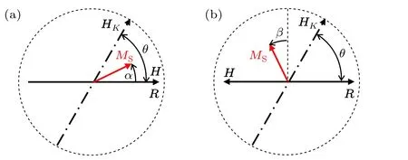
Fig. 1. Schematic illustration of SW particle. (a) The applied magnetic field H is parallel to the reference axis R in the magnetizing process,(b)the magnetization reversal process where H is antiparallel to the reference axis R.

This paper directly shows the analytic solution ofθ(the angle between the anisotropy fieldHKand the reference axisR) varying withα(the angles between the saturation magnetizationMSand the reference axisR) by using the antitrigonometric function. Due to the anti-trigonometric functiony=f(x) is symmetric abouty=x, the relation ofα～θat different applied magnetic fields is also exposed. Then, the hysteresis loops magnetized in any direction are obtained by usingM=MScosα. Using these loops, the hysteresis loops are obtained in the randomly oriented and non-interacting SW particle ensembles. Finally,the correctness of the analytic solution is verified by fitting the exact solutions of remanence,switching field and coercivity.

2. Anisotropy free energy density

The spherical SW particle is shown in Fig. 1. The total free energy densityFincluding Zeeman energy and anisotropy energy. For the magnetizing and magnetization reversal processes,Fcan be expressed as

whereKis the anisotropy constant,µ0is the vacuum permeability,MSis the saturation magnetization, andHis the applied magnetic field.θis the angle between the anisotropy fieldHKand the reference axisR,andα(β)is the angle between the saturation magnetizationMSand the reference axisR(the perpendicular direction of the reference).The stable direction of saturation magnetization can be determined by the minimum of the free energy density

3. The anti-trigonometric solution of α ～θ

It can be directly obtained from Eqs.(2a)and(3a)

Letθ(α)=f(α) andθ(β)=g(β). The anti-trigonometric solution ofαcan be directly obtained from Eqs.(4a)and(4b)

The former and latter reflect the solution of the magnetizing and magnetization reversal processes,respectively. Determining all possible stable solutions in Eqs. (4a) and (4b) are the key to obtain the magnetizing curves and hysteresis loops using Eqs.(5a)and(5b).

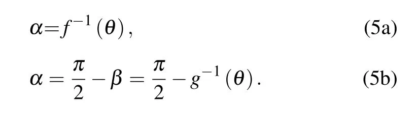
It is known that the domain of they= arcsin(x) is[-1,1], and the range is [-π/2,π/2].[30]It can be seen that the domain of Eqs. (4a) and (4b) satisfies-1≤2hsinα ≤1 and-1≤2hcosβ≤1, respectively. Then their ranges are-π/4≤(θ-α)≤π/4 and-π/4≤(θ-β)≤π/4. Because(θ-α)is the angle between the saturation magnetization and the anisotropy field, we can obtain the solution in-π/4≤(θ-α)≤π/4 by Eq. (4a), as shown in the grey area I of Fig.2. Consideringβ=α-π/2,we can obtain the solution in-3π/4≤(θ-α)≤-π/4 by Eq. (4b), as shown in the yellow area I of Fig. 2. If we consider another direction of the anisotropy field where the magnetization deviates from the easy axis,Eqs.(4a)and(4b)can describe the gray and yellow areas II in Fig. 2, respectively. Therefore, Eqs. (4a) and (4b)completely describe the magnetization deviating from the easy axis in the SW model under the applied magnetic field in the entire space.

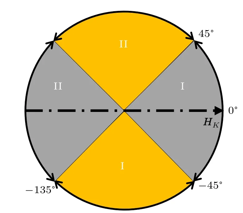
Fig. 2. The solution of Eqs. (4a) and (4b). I and II represent the results of the magnetization deviating from the anisotropy field HK and-HK,respectively. The gray and yellow areas represent the results of magnetizing and magnetization reversal,respectively.

The relation curve ofθ～αcan be obtained by Eqs.(4a)and (4b), as shown in Fig. 3(a). The solid line and the dotted line respectively represent theθ=f(α) andθ=g(β),whenθis limited in [0,π/2]. As the reduced fieldhchanging in [-∞,-1] and [-0.5,∞], the solutions of Eqs. (4a) and(4b) show a continuous curve ofθ～α. Moreover, it is not a continuous curve ofθ～αwhenhchanges in (-1,-0.5),as shown by the curve ofh=-0.6 and-0.75 in Fig.3(a). It is because that the magnetization will jump whenhchanges in(-1,-0.5).[22,23]The position(α,θ)of the horizontal tangent of the curve corresponds to the unstable position under the switching fieldhSW. According to the definition of the anti-trigonometric function,[30]the functionα=f-1(θ) can be obtained by symmetrically transformingθ=f(α) with a straight lineθ=α. This result can be used to obtain the stable magnetization angleαwhen the applied magnetic field changes under a given applied field angleθ.

Fig. 3. The relation curve of θ ～α with different reduced fields h as 1.5,0.75, 0.6, 0, -0.5, -0.6, -0.75, and-1.5, respectively. The solid line and the dotted line are the solutions of Eqs.(4a)and(4b),respectively.

4. Hysteresis loops

Let the direction of reference axisRbe the initial direction ofH. The hysteresis loop is the projection of the magnetization in the reference axis direction. In a uniaxial system,whenHchanges,the deviation of the magnetization from the easy axis involves two anisotropy field directions.If the angles betweenHand the two anisotropy fields are the same,the angle of the magnetization deviating from the easy axis is equal.Therefore,we only need to deal with one case where the magnetization deviates from an anisotropy field. Another case can be described in the hysteresis loop through an inversion center of the previous result.

For the first case, the relation curve of cosα～θunder different reduced fieldshin the reference directionRcan be obtained by using the functionα=f-1(θ), as shown in Fig.4(a). For any given applied field angleθ,cosα=M/MSunder different reduced fieldshis obtained on the cosα～θcurve in the order of reduced fieldhfrom large to small and from positive to negative. Then we plot the points of(h,M/MS) in sequence to get the magnetizing and magnetization reversal curves. Figure 4(b)shows the relation curve ofM/MS～hatθ=16.6°and 73.4°. To demonstrate this idea,we takeθ=73.4°as an example to illustrate the specific process. The points A, B, C1,2, and D correspond to the points(h,M/MS)underh=1.5,0,-0.6,and-0.5 in Figs.4(a)and 4(b). C1and C2are the points before and after the magnetization jump under the switching fieldhSW=-0.6. Then,in the coordinate system withM/MSas the vertical axis andhas the horizontal axis. We can draw points from A, and then draw the remaining(h,M/MS)points in descending order of the reduced fieldh,including the remanence B underh=0 and C1and C2under switching fieldhSW=-0.6. Finally,we draw to D.Connect all the points into a line to get the magnetizing and magnetization reversal curves of the first case,as shown in the red solid line of Fig.4(b).The red dotted line in Fig.4(b)is the center inversion of the first case. It is worth noticing that there is no saturation magnetization in the magnetic moment at other applied field angles, except forθ=0°and 90°. This model can also be used to judge the stable magnetization position and saturation magnetization in the measurement of soft magnetic high-frequency[11]and magnetoelectric transport.[17]

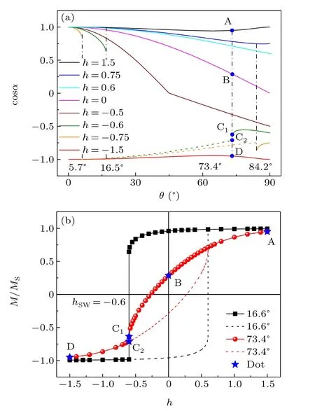
Fig. 4. (a) The relation curve of cosα～θ with different reduced fields h as 1.5, 0.75, 0.6, 0, -0.5, -0.6, -0.75, and -1.5. The dotted line is the relation curve of cosα～θ after the magnetization jumps under hSW, which is equal to the relation curve of -cosα～θ under -hSW. (b) The hysteresis loop at θ =16.6° and 73.4°. The points A,B,C1,2 and D in panels(a)and(b)correspond to the points(h,M/MS)under h=1.5,0,-0.6,and-0.5 at θ =73.4°.

5. Randomly oriented and non-interacting SW particle ensembles

Fig. 5. (a) Schematic illustration of the SW particle ensembles in a twodimensional(2D)plane. The distribution of SW particles at different angles θ is uniform. (b) The SW particles are not uniformly distributed as the angle θ increases in three-dimensional(3D)systems. (c)The hysteresis loops of SW particle ensembles and the blue dotted line is given by Stoner and Wohlfarth in 1948.

Based on the relation curve ofM/MS～θ, the representative hysteresis loops of the randomly oriented and noninteracting SW particle ensembles can be obtained.Because of the different distribution of SW particles in different dimensions, we use two different averaging methods to deal with.For the first case, the distribution of SW particles in all directions is equal with the increase ofθin a 2D plane. Then,we divide the central angle intonparts(n →∞)along the direction ofH, and each part is Δθ. The length of the circle is also divided intonparts,and each arc length is ΔL=RΔθ,as shown in Fig. 5(a). According to the symmetry of the SW model,[1]the hysteresis loop ofθin the interval [0,π] and[π,2π] is equal. Therefore, the hysteresis loops of the SW particle ensembles can be obtained inθ ∈[0,π]

M(h)iis the magnetization under the reduced fieldhat the applied field angleθ, and Δθis the adjacent angular interval.Another situation is in a 3D sphere. The associated revolution surface will be larger as the angleθincreasing in the range ofθ ∈[0,π/2],so SW particles do not have the same number in every direction. In order to solve this problem,the central angle is equally divided intonparts(n →∞). The sphere is also divided intonslices at the same time, as shown in Fig. 5(b).Then the peripheral area of a thin slice is Δs=2πR2sinθΔθ(θ∈[0,π]), the hysteresis loops in the plane could be refined following spheroidal-based weighting[1,31]

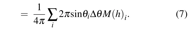
θiis the angle betweenHand the anisotropic fieldHkiat positioni. A total of 540 equiangular spaced(Δθ=0.33°)hysteresis loops of the applied field angleθfrom toπcan be obtained by Eqs. (6) and (7) as shown in Fig. 5(c). The red line represents the hysteresis loop of SW particle ensembles in a two-dimensional plane,and the black line is the result in a three-dimensional sphere. It completely coincides with the result given by Stoner and Wohlfarth in 1948.[1]

6. Verifying the correctness of the analytic solution

In order to verify the correctness of the above analytic solution,we fit the numerical solutions of remanence,switching field and coercivity with the exact solutions. It is known that the remanenceMris the projection of the magnetization in the initial direction ofHwhenHdrops from the saturation magnetization to zero,[32]

Based on the relation curve of cosα～θ,the numerical solutions of coercivity,switching field,and remanence also can be obtained in different applied field directions, as shown in the dot of Fig.6. Moreover,the numerical solutions can be completely fitted with Eqs. (8)-(10), as shown in Fig. 6, which verifies the correctness of the analytic solution.

Fig. 6. The numerical (dot) and exact (line) solutions of coercivity, remanence,and switching field.

7. Conclusion

We divide the stable position where the magnetization deviates from the easy axis into two regions based on the difference between magnetizing and magnetization reversal processes and obtain the analytic solutions in the entire space by the anti-trigonometric function. Based on the relation curve ofθ～α, cosα～θunder different reduced fieldhcan be obtained, and then the hysteresis loops under any applied field angle can be obtained. In addition, the hysteresis loops with the easy axis of the non-interacting SW particle ensembles randomly orienting in two dimensions and three dimensions also can be obtained by the relation curve of cosα～θ. The results of remanence,switching field,and coercivity obtained by the analytic solution are consistent with the exact solutions of the above three physical quantities. The analytic solution of the SW model is of great help to understand the actual magnetization reversal mechanism of SW particles.

Acknowledgments

Project supported by the National Natural Science Foundation of China (Grant Nos. 91963201, 12174163, and 12075102), PCSIRT (Grant No. IRT-16R35), and the 111 Project(Grant No.B20063).