Hydrodynamic Instability Analysis of the Axial Flow Pump in an Ethylene Polymerization Loop Reactor

Lu Jin; Yang Yao; Sun Jingyuan; Huang Zhengliang; Yang Yongrong; Wang Jingdai

(1. Zhejiang Provincial Key Laboratory of Advanced Chemical Engineering Manufacture Technology,College of Chemical and Biological Engineering, Zhejiang University, Hangzhou 310058;2. State Key Laboratory of Chemical Engineering, College of Chemical and Biological Engineering, Zhejiang University, Hangzhou 310058)

Abstract: The hydrodynamic instability of the axial flow pump in a loop reactor has long been a troubling issue to be solved in the polyethylene industry due to the lack of a better mechanismic understanding. Generally, the instability of an axial flow pump can be reflected by the fluctuation of the pump head. In this study, the transient computational fluid dynamics (CFD)simulation is adopted to study the hydrodynamic instability of the axial flow pump used in an ethylene polymerization loop reactor. The results show that the pump head under single liquid phase nearly remains constant while the pump head under slurry phase fluctuates due to the variation of solid volume fraction distribution in the pump. Besides, under the combined effect of the maximum solid volume fraction difference in the pump and the turbulence intensity of the liquid phase, the fluctuation of the pump head under slurry phase increases when the solid volume fraction in the loop reactor increases from 0.10 to 0.29, and the fluctuation decreases, when the solid volume fraction increases from 0.29 to 0.35. Furthermore,there is a negative correlation between the pump head and the solid volume fraction in the pump; with the increase of solid volume fraction in the loop reactor, and the correlation coefficient increases as well. Moreover, a ‘spiral particulate band’ phenomenon is formed in the ascending leg caused by three mechanisms, viz.: the segregation of particles in all bends, the dispersion of particles by the secondary flow in the ascending leg, and the rotational movement of particles in the pump.

Key words: axial flow pump; loop reactor; CFD; hydrodynamic instability; polyethylene

1 Introduction

In the field of polyolefin production, loop reactors are widely used because of their simple structure, high space-time yields,and easy heat removal[1-2]. In a typical ethylene polymerization loop reactor, the reactants are present in liquid state while the solid polymer particles suspend in the liquid, resulting in liquid-solid slurry flows. Driven by the axial flow pump, the slurry flows circulate inside the loop reactor. The axial flow pump is the only core power equipment in the loop reactor,thus, the stable operation of the pump is crucial to the stable operation of the loop reactor. However, industrial operations show that, under high particle concentration conditions, the pump power may increase sharply and fluctuate violently,indicating an obvious instability of reactor operation. This unstable phenomenon, named ‘pump power swelling’ by Fouarge in the literature[3-5], is a troubling issue to be solved in the polyethylene industry due to the lack of mechanismic understanding. Therefore, it is significant to explore the reasons for the hydrodynamic instability of axial flow pumps.Generally, the operating stability of an axial flow pump is affected by the fluid flow at the inlet and outlet of the pump. In an ethylene polymerization loop reactor,both the inlet and outlet of the pump are connected with the loop reactor. Thus, it is necessary to study the flow characteristics of the slurry in the loop reactor. Shi, et al.[6]adopted the CFD simulation to study the steadystate liquid-solid flow in a propylene polymerization loop reactor. The results showed that the distribution of solid particles in the straight pipe became more uniform, when the particle size decreased and the circulation velocity of the slurry flow increased. Yan, et al.[7]coupled CFD with the population balance model (PBM) to describe the steadystate liquid-solid flow in a 2D propylene polymerization loop reactor. The results showed that a larger mean particle diameter and a broader particle size distribution would form a less uniform slurry velocity distribution. In addition,Yan, et al.[8]adopted the steady-state CFD simulation to investigate the effect of guide vane on the flow behaviors in a loop reactor. The results revealed that adding a guide vane weakened the turbulent intensity, reduced the component of the rotational velocity, and contributed to the uniform distribution of the particles in the reactor.

However, compared with the steady-state CFD simulation,the transient CFD simulation is more suitable for describing the dynamic behavior of slurry flows in loop reactors. Li, et al.[9]adopted the transient CFD simulation to describe the slurry flows in an 8-leg loop reactor. The results showed that the competition between the segregation and dispersion mechanisms can generate multiple slurry clusters, and the slurry clusters may eventually develop into large slugs after a long period of circulating flow in the loop reactor.Furthermore, Li, et al.[10]found that the appearance of the slug made the pressure output of the axial flow pump fluctuate greatly. However, there is no direct evidence of the existence of slugs in loop reactors, so the appearance of slugs may not be the accurate reason for the unstable phenomenon of the axial flow pump.

Except for the characteristics of slurry flows in loop reactors, the characteristics of liquid-solid flows in axial flow pumps also needed to be studied to figure out the reason for the unstable phenomenon of axial flow pumps.Yan, et al.[11]adopted the steady-state CFD simulation to describe the liquid-solid flows in an axial flow pump. The results showed that the pump head decreased with the increase of the solid volume fraction, resulting in energy allowance in the loop reactor, which may be one of the main causes of power fluctuation in the axial flow pump.However, Yan, et al.[11]ignored the influence of the slurry flow in the loop reactor on the characteristics of the slurry flow in the axial flow pump.

In this work, the hydrodynamic instability of an axial flow pump in a loop reactor is studied. The transient Eulerian-Eulerian two-fluid model incorporated with the kinetic theory of granular flow (KTGF) is adopted to simulate the liquid-solid flows in the loop reactor. The hydrodynamic instability of the pump is analyzed from the perspective of the pump head fluctuation. Firstly, the influence of solid particle distribution in the pump on the pump head is investigated. Secondly, the influence of solid volume fraction in the loop reactor on the pump head is studied.Finally, the influence of the axial flow pump on the slurry flow in the ascending leg is discussed.

2 Equations of Model

In this paper, the slurry flow behaviors inside a loop reactor are described by a transient Eulerian-Eulerian two-fluid model, which takes the assumption that the liquid phase is incompressible and the solid phase is a kind of continuous fluid. The flow behaviors of the solid phase are described by the kinetic theory of granular flow, where the parameters associated with the solid phase are estimated by the solid temperature. In addition, the momentum exchange between the liquid phase and solid phase is described by the empirical drag law proposed by Gidaspow, et al.[7,12]. Equations of CFD models used in this work are listed in Table 1.

Table 1 Equations of CFD models

Table 1 Equations of CFD models (continued)

3 Numerical Model

3.1 The two-leg loop reactor

In this study, an industrial-scale two-leg loop reactor is taken into consideration, as shown in Figure 1. As illustrated in Figure 1 (a), the reactor consists of a 180°bend (R1= 1.32 m), a 90° bend (R2= 0.66 m), two vertical legs (L1= 12.4 m), an axial flow pump, and a horizontal pipe (L2= 1.36 m). The inner diameter (D) of all pipes is 0.33 m. Note that the inlets and outlets of the loop reactor are neglected since the infusing and withdrawing rates are much smaller than the circulating rate of the slurry.

Figure 1 (b) shows the detailed view of the axial flow pump, which consists of an impeller and an outlet channel. Figure 1 (c) shows the detailed view of the impeller, which is composed of a hub and four blades.Each blade consists of two surfaces, i.e., a suction surface(S), and a pressure surface (P).

Figure 1 The two-leg loop reactor: (a) Geometry of the reactor; (b) The detailed view of the axial flow pump; (c)The detailed view of the impeller

The physical properties of the slurry in the loop reactor are listed in Table 2, in whichρandμdenote the density and viscosity, respectively, and the subscripts ‘s’, ‘i’, and‘w’ represent solid particles, liquid isobutane, and liquid water, respectively. The average diameter of polymer particles is measured to bedp= 0.5 mm, which is a typical grade for PE products[9]. In this paper, five groups of solid volume fractions (αs) in the loop reactor are considered:αs= 0.10, 0.15, 0.24, 0.29, and 0.35.

Table 2 Physical properties of the solid and liquid phase

3.2 Boundary conditions and model setup

The rotational speed of the pump is specified at 1448 r/min.The wall boundary conditions are applied to the impeller and all pipes in the loop reactor. The roughness of all walls is specified at 3.2 μm. For these wall boundaries,the solid phase is provided with the partial slip condition proposed by Johnson and Jackson[18-19], while the liquid phase is provided with the no-slip condition. The particles are uniformly distributed in the loop reactor at the initial stage.

The governing equations shown in Section 2 are all solved by the transient pressure-based solver provided by the commercial CFD package ANSYS Fluent 18.0 with double precision mode. The velocity and pressure terms in the Navier-Stokes equations are coupled with the Phase Couple SIMPLE scheme. The RNG k-ε model is selected to describe the turbulent flow as it enhances the prediction of swirling flows based on the standard k-ε model. The motion of the axial flow pump is simulated by the Multiple Reference Frame (MRF) model in Fluent[9]. After performing a mesh independence study,a computational mesh consisting of approximately 2.1 million computational cells is adopted in this study.

The simulation times in all cases are set longer than 50 s,which is approximately 10 flow cycles of the loop reactor.The computational results after 50 s are presented and discussed in Section 4.

4 Results and Discussion

4.1 Model verification

The axial flow pump is the core equipment for circulating the slurry in the loop reactor[20]. Therefore, the calculation accuracy of the axial flow pump is significant for the prediction of the slurry flows in the loop reactor. We compare the pump head under clear water conditions predicted by CFD simulation with that measured by experiment in the manufacturing factory. It is found that the predicted pump head agrees well with the experimental data, as shown in Figure 2. Thus, the accuracy of the CFD simulation is validated.

Figure 2 Pump head characteristic curve of axial flow pump under clear water condition

In addition, according to Yan[8], the numerical model for simulating liquid-solid flows in the loop reactor can be validated by comparing the pressure gradient obtained by the CFD simulation with that predicted by classical Newitt model[21]. According to the Newitt’s correlation,the pressure gradient is written as

whereflis the friction factor of the liquid,dprepresents the average diameter of particles.

As shown in Table 3, the absolute relative errors between the pressure gradient obtained by the CFD simulation and that calculated by the Newitt’s correlation (see Eq. (1))are all less than 2%. Therefore, the numerical model in this paper is capable of accurately predicting the liquidsolid flow behaviors in the loop reactor coupled with an axial flow pump.

Table 3 The pressure gradient obtained by CFD simulation and that calculated by Newitt’s correlation.

4.2 Influence of solid particle distribution in the pump on the hydrodynamic instability

Based on the verification of the numerical model in Section 4.1, the influence of the distribution of solid particles in the pump on the hydrodynamic instability of the axial flow pump is investigated in this section.

In industry, the stability of an axial flow pump can be reflected by the fluctuation of the pump power[22].The stability is considered as becoming worse, if the fluctuation of the pump power becomes stronger. To some extent, the fluctuation of the pump power is reflected by the fluctuation of the pump head. Therefore, in this paper,we take the fluctuation of the pump head as the evaluation index for studying the hydrodynamic instability of the axial flow pump. The standard deviation of the pump head is used to evaluate the fluctuation of the head.

The actual pump head is calculated by the following equation:

where the subscripts ‘in’ and ‘out’ denote the inlet and outlet of the pump, respectively, and ΔZdenotes the height difference between the inlet and outlet of the pump, as shown in Figure 1 (b).

The theoretical head of the pump can be obtained by the following equation:

whereuis the peripheral velocity,vu2is the projection of the liquid velocity at the impeller outlet in the direction of velocityu,vu1is the projection of the liquid velocity at the impeller inlet in the direction of velocityu.

Figure 3 shows the curves ofHa/Htwith respect to time under conditions covering single-phase water, singlephase isobutane, and isobutane-polyethylene slurry flow(αs= 0.24), respectively. It can be found that, among these three conditions, the pump head under the isobutane condition is the maximum, while the pump head under the isobutane-polyethylene condition is the minimum.The differences in pump head are mainly caused by the differences in viscosity of the fluid. The viscosity of isobutane is smaller than that of water, so the hydraulic loss of the axial flow pump under isobutane conditions is smaller than that under water conditions. Therefore,the pump head under isobutane conditions is higher than that under water conditions. Besides, the addition of solid particles increases the viscosity of the liquid-solid flow and thus the pump head decreases. In addition, a large amount of energy loss is caused by the collision of particles and the pump, leading to a further reduction of the pump head.

Figure 3 Fluctuation curve of Ha/Ht for different fluid media under the same volume flow rate of 2460 m3/h

Table 4 Average value and standard deviation of the pump head

The average values and standard deviations of the pump head are presented in Table 4. It can be found from Figure 3 and Table 4 that the pump head under water and isobutane conditions nearly remains constant, while the pump head under isobutane-polyethylene condition fluctuates violently. Therefore, the addition of solid particles leads to the hydrodynamic instability of the axial flow pump.In order to clarify the reasons for the fluctuation of the pump head under slurry flow condition as shown in Figure 3, we compare the liquid velocity field under the single-phase isobutane condition with that under the isobutane-polyethylene slurry flow (αs= 0.24) condition.The cylindrical surface shown in Figure 4 is selected as an observation surface in the pump. The fluid velocity fields of this cylindrical surface corresponding to the four points(Pa1,Pa2,Pb1, andPb2) in Figure 3 are presented in Figure 5.It can be found that, on the one hand, the addition of solid particles has an important influence on the distribution of fluid velocity in the pump, and makes the fluid velocity field more nonuniform. On the other hand, the fluid fields of pointsPb1andPb2are very close, while the fluid fields of pointsPa1andPa2are quite different, especially in the regions within the black rectangle. Therefore,the variation of fluid velocity in the pump leads to the fluctuation of the pump head from pointPa1to pointPa2,as shown in Figure 3.

Figure 4 Illustration of a cylindrical surface as an observation surface

The solid volume fraction of the cylindrical surface (see Figure 4) corresponding to the two pointsPa1andPa2in Figure 3 is presented in Figure 6. It can be found that the distribution of particle concentration is nonuniform.In addition, the solid volume fraction of pointPa1is quite different from that of pointPa2, especially in the regions within the black rectangle. Moreover, upon comparing the solid volume fraction and fluid velocity fields of pointsPa1andPa2, as shown in Figure 5 and Figure 6, the regions where the solid volume fraction clearly differs would overlap the regions where the fluid velocity field distinctly differs. Therefore, it can be concluded that the variation of solid volume fraction distribution in the pump leads to the variation of the fluid velocity field, and would further result in the fluctuation of the pump head from pointsPa1toPa2, as shown in Figure 3.

Figure 5 Fluid velocity field of the cylindrical surface corresponding to four points in Figure 3: (a) Pa1; (b) Pa2; (c) Pb1; (d) Pb2

Figure 6 Solid volume fraction of the cylindrical surface corresponding to two points in Figure 3: (a) Pa1; (b) Pa2

4.3 Influence of particle concentration in the loop reactor on the hydrodynamic instability

As discussed in Section 4.2, upon comparing with the single-phase isobutane condition, the addition of solid particles leads to the fluctuation of the pump head, i.e.,the hydrodynamic instability of the axial flow pump. To investigate the influence of particle concentration in the loop reactor on the hydrodynamic instability of the pump,five groups of solid volume fractions (αs=0.10, 0.15,0.24, 0.29, and 0.35) in the loop reactor are tested in this section.

4.3.1 Fluctuation of the pump head

Figure 7 shows the standard deviation of the pump head within 40 s under different solid volume fractions (αsin the loop reactor). It can be found that when theαsdoes not exceed 0.24, the standard deviation of the pump head grows slowly with the increase ofαs. Whenαsincreases from 0.24 to 0.29, the standard deviation increases sharply from 0.28 m to 0.50 m. However, with the further increase ofαs, the standard deviation dramatically decreases and reaches the minimum value.

Figure 7 Standard deviation of pump head under different solid volume fractions (αs)

4.3.2 Fluctuation of solid volume fraction in the pump The fluctuation of solid volume fraction in the axial flow pump is discussed in this section. Compared with the flow behavior in other regions of the pump, the flow behavior at the blades is more complex and has a greater influence on the fluctuation of the pump head.Therefore, the fluctuation of solid volume fraction on the blades is analyzed. One of the four blades is taken as an example, as shown in Figure 8. Five streamlines are uniformly selected on both sides of the blade.We useSiSandSiP(i=1, 2, 3, 4, 5) to denote theith streamline on the suction surface and pressure surface,respectively.

Figure 8 Illustration of streamlines

Figure 9 shows the average standard deviation of the solid volume fraction of all streamlines on the blade within 20 s under different solid volume fractions (αs) in the loop reactor, which reflects the overall fluctuation of the solid phase on the blade. It can be found that whenαs＜ 0.29,the average standard deviation generally increases with the increase of αs. However, whenαs＞ 0.29, the average standard deviation decreases.

Figure 9 Relation between the average standard deviation of solid volume fraction of all streamlines on the blade and the solid volume fraction in the loop reactor

In order to figure out the reasons for the changing trend of the curve in Figure 9, both the maximum solid volume fraction difference on the blade and the turbulence intensity in the loop reactor are investigated.

Figure 10 shows the time-averaged distribution of solid volume fraction at four typical streamlines, i.e.:S1S,S1P,, andS5P(see Figure 8) on the blade of the axial flow pump within 20 s. It can be found that the solid volume fraction on the pressure surface of the blade is larger than that on the suction surface. This outcome can be related to different forces applied to the particles on the pressure surface and suction surface. At the suction surface of the blade, the slurry is sucked into the suction surface due to the pressure difference. It is more difficult for particles to be sucked than the liquid isobutane, because particles have higher inertia caused by their higher density.Besides, at the pressure surface of the blade, the slurry is pushed out of the impeller along the axial direction. It is more difficult for particles to be pushed out than the liquid isobutane due to their higher inertia. Therefore,it is easier for particles to be gathered on the pressure surface than the suction surface, resulting in a higher solid volume fraction on the pressure surface than on the suction surface.

In addition, Figure 10 shows that the solid volume fraction increases fromS1toS5. Because the density of solid particles is higher than that of liquid isobutane,the centrifugal force on the particles is greater than that on the liquid isobutane, which makes the solid particles more easily to leave away from the hub than the liquid isobutane[23-24]. Then, the particles would gather at the tip of the blade due to obstruction of the pump shell.

It can be seen from Figure 10 that the distribution of solid volume fraction on the blade is nonuniform.Generally, a higher solid volume fraction difference leads to a higher standard deviation of solid volume fraction. The maximum solid volume fraction difference of all streamlines, i.e., the maximum solid volume fraction of all streamlines minus the minimum one under different solid volume fractions (αs) in the loop reactor is shown in Figure 11. It can be found that, with the increase of αs, the maximum solid volume fraction difference on the blade becomes higher. A higher maximum solid volume fraction difference may lead to a higher standard deviation of the solid volume fraction.However, the fluctuation of the solid volume fraction on the blade is affected not only by the maximum solid volume fraction difference but also by the turbulence intensity of the liquid, which will be discussed in the following paragraph.The average fluid velocity in each leg of the loop reactor is shown in Figure 12. It can be found that as the solid volume fraction (αs) in the loop reactor increases, the average liquid velocity in both legs gradually decreases,which means that the turbulence intensity of the liquid phase gradually decreases as well, as shown in Figure 11.Figure 13 shows the liquid streamline and solid volume fraction distribution on the plane M (see Figure 1 (a))in the loop reactor under differentαs, where the distance between the plane M and the outlet plane of the 180° bend isLm= 1.0 m. It can be found that the liquid streamline structure becomes simpler with the increase ofαs, which also reflects the decrease of the turbulence intensity of the liquid flow, as shown in Figure 11.

Figure 10 Time-averaged distribution of solid volume fraction at four typical streamlines on the blade within 20 s

Figure 11 Turbulence intensity and maximum solid volume fraction difference of all streamlines

Under the two influence factors, i.e., the solid volume fraction difference and the turbulence intensity of the liquid phase, as shown in Figure 11, the average standard deviation of solid volume fraction in Figure 9 increases with the increase ofαswhenαs＜ 0.29, and then decreases whenαs＞ 0.29.

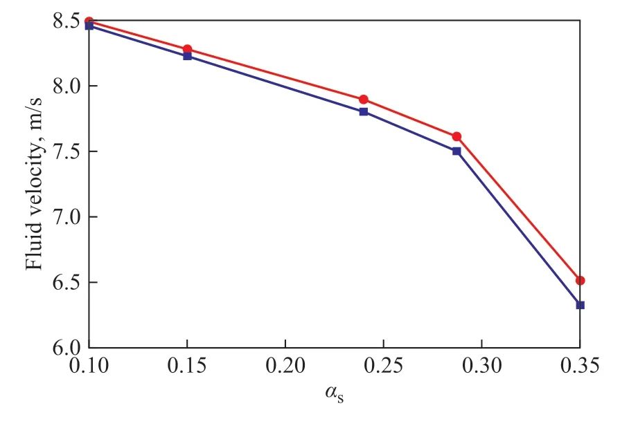
Figure 12 Average fluid velocity in each leg of the loop reactor

Upon comparing Figure 7 and Figure 9, the variation trend of the standard deviation of the pump head agrees well with the variation trend of the average standard deviation of the solid volume fraction in the pump,which indicates that the fluctuation of the pump head is governed by the fluctuation of the solid volume fraction in the pump. To further prove this conclusion, the dynamic correlation between the solid volume fraction in the pump and the pump head is discussed in Section 4.3.3.

4.3.3 Dynamic correlation between the pump head and the solid volume fraction in the pump

As shown in Figure 14, the plane N in the pump is selected as a monitoring plane. Figure 15 shows the curves of the average solid volume fraction on the plane N and the pump head with respect to time. It can be found that the average solid volume fraction on the plane N is negatively correlated with the pump head. Table 5 shows the Pierre correlation coefficient of these two variables under different solid volume fractions (αs) in the loop reactor. Asαsincreases, the negative correlation coefficient increases as well. When theαsis equal to 0.29,the Pierre correlation coefficient of these two variables is-0.8, indicating that they are significantly correlated. In the isobutane-polyethylene system, a higher solid volume fraction in the loop reactor leads to a higher viscosity of the slurry flow, and can further result in a lower pump head. Therefore, the pump head and the average solid volume fraction in the pump are negatively correlated.The dynamic correlation between these two variables further proves that the fluctuation of the pump head is governed by the fluctuation of the solid volume fraction in the pump, as discussed in Section 4.3.2.

Figure 13 Liquid streamlines and solid volume fraction distribution on the plane M at different αs

Figure 14 The illustration of plane N

Figure 15 The pump head and the average solid volume fraction on the plane N (αs = 0.29)

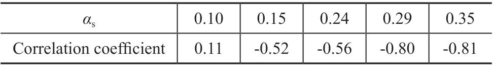
Table 5 Pierre correlation coefficient of the pump head and the average solid volume fraction on the plane N

4.4 Influence of axial flow pump on slurry flow in the ascending leg

The hydrodynamic instability of the axial flow pump with different solid volume fractions (αs) in the loop reactor has been analyzed in Section 4.2 and Section 4.3. In this section, the influence of the axial flow pump with different degrees of hydrodynamic instability on the slurry flow in the loop reactor at differentαsis studied.The ascending leg, which is adjacent to the outlet of the axial flow pump, is selected as the observation leg since the pump has more influence on the ascending leg than on the descending leg and other pipes.

Figure 16 shows the contour plots of solid volume fraction at different positions in the ascending leg whenαs= 0.29. Specifically, Figure 16 (a) shows the contour on the inner wall of the ascending leg, and Figure 16 (b)shows the contour at corresponding cross-sectional planes in Figure 16 (a). It can be found that there is a particulate band with a certain thickness in the ascending leg. The particulate band spirals in the ascending leg and rotates in a clockwise direction consistent with the direction of impeller rotation. The particulate band is formed due to the segregation of particles in all bends and the dispersion of particles by the secondary flow in the vertical legs[9].Then after obtaining a large angular velocity due to the rotation of the pump, the solid phase rotates in the ascending leg. Finally, with the development of the flow,the ‘spiral particulate band’ is formed, as shown in Figure 16 (a).

Figure 16 Contour plots of solid volume fraction indifferent positions of the ascending leg (αs=0.29): (a) on the inner wall of the pipe; (b) on the cross-sectional planes.

Figure 17 shows the solid volume fraction distribution in the ascending leg under different solid volume fractions(αs) in the loop reactor. It is found that with the increase ofαs, the spiral particulate band becomes thicker, and the number of complete spiral structures increases. There are two reasons for this phenomenon. Firstly, with the increase ofαs, the segregation of solid particles increases and the dispersion of solid particles decreases, thus, the spiral particulate band becomes thicker. Secondly, with the increase of αs, the rotational velocity of the slurry flow remains nearly unchanged since the rotational speed of the pump is constant, while the axial velocity of the slurry flow in the ascending leg decreases (see Figure 12). Therefore, the number of complete spiral structures increases.

Figure 18 shows the curve of solid volume fraction at point P (see Figure 16 (b)) with respect to time. It can be found that there are periodic fluctuations of the solid volume fraction at point P, which can be regarded as a periodic movement of the particulate band. In addition,it can be found that the fluctuation period of the solid volume fraction at point P is aroud 5 s, which is consistent with the fluctuation period of the solid volume fraction on the plane N, the fluctuation period of the pump head (see Figure 15), and the cycle of slurry circulation.

5 Conclusions

In this work, we apply CFD simulations using the transient Eulerian-Eulerian two-fluid method to study the hydrodynamic instability of the axial flow pump inside an industrial-scale two-leg loop reactor. The following conclusions can be made:

1) The numerical model is validated by comparing the pump head calculated by CFD simulation with that measured by experiments and comparing the pressure gradient obtained by CFD simulation with that calculated by the Newitt’s correlation.

Figure 17 Contour plots of solid volume fraction in the ascending leg at different αs in the loop reactor

Figure 18 Fluctuation of solid volume fraction at point P(see Figure 16 (b))

2) The influence of the solid particle distribution in the pump on the hydrodynamic instability of the pump is investigated. The pump heads under isobutanepolyethylene slurry flow conditions are lower than those under single-phase isobutane conditions. In addition, the variation of solid volume fraction distribution in the pump under slurry flow conditions leads to the fluctuation of the pump head.

3) As the solid volume fraction in the loop reactor increases, the maximum solid volume fraction difference in the pump increases as well, but the turbulence intensity of the liquid phase decreases. Under the above two influence factors, the pump head increases at first with the increase of the solid volume fraction in the loop reactor until the solid volume fraction reaches 0.29; afterward,the pump head gradually decreases. In addition, there is a negative correlation between the pump head and the solid volume fraction in the pump, and the correlation coefficient increases with an increasing solid volume fraction in the loop reactor.

4) A ‘spiral particulate band’ is formed in the ascending leg due to three competitive mechanisms: the segregation of particles in all bends, the dispersion of particles by the secondary flow in the ascending leg, and the rotational movement of particles in the pump. As the solid volume fraction in the loop reactor increases, the spiral particulate band becomes more obvious. In addition, the fluctuation period of the solid volume fraction of particles in the spiral particulate band is consistent with the fluctuation period of the pump head and the period of slurry circulation.

Acknowledgments:The authors gratefully acknowledge financial supports from Projects of the National Natural Science Foundation of China for Young (No. 21808198), the Major Research Project of National Natural Science Foundation of China (No. 91834303), the Science Fund for Creative Research Groups of National Natural Science Foundation of China (No.61621002).