Residual field suppression for magnetocardiography measurement inside a thin magnetically shielded room using bi-planar coil

Kang Yang(杨康)， Hong-Wei Zhang(张宏伟)， Qian-Nian Zhang(张千年)，Jun-Jun Zha(查君君)， and Deng-Chao Huang(黄登朝)，†

1College of Electrical Engineering，Anhui Polytechnic University，Wuhu 241000，China

2Key Laboratory of Advanced Perception and Intelligent Control of High-end Equipment，Ministry of Education，Anhui Polytechnic University，Wuhu 241000，China

Keywords: SQUID，magnetocardiography，bi-planar coil，active compensation

1. Introduction

Magnetocardiography (MCG) is a non-invasive imaging tool to measure and analyze the magnetic field generated from human heart activity， whose intensity is typically as low as several tens of pico-Tesla(pT).It has been verified by clinical trials that MCG can be a potential technique for heart disease diagnosis.[1，2]However，because of the inevitable environmental magnetic noise， whose intensity can reach up to several hundred micro-Tesla (μT)， it is a huge challenge to obtain MCG signals if the extremely sensitive superconducting quantum interference devices (SQUIDs) are only utilized.[3，4]To suppress the environmental disturbance，many research groups have attempted various shielding techniques，such as magnetically shielded rooms(MSRs)，hardware or software gradiometers，and signal post-processing algorithms.[5，6]Typically，the most straightforward and effective way to restrain the environmental field noise is using the MSR. But the high cost and large size of a strongly MSR limits the clinical application of the MCG technique. Furthermore， the gradiometer or signal post-processing method has the disadvantage of attenuating the useful signals when suppressing the dominant environmental noise.

To control the MSR building costs while guarantee the MCG signal quality， active compensation method combined with a thin passive MSR seems to be a considerable compromise.[7，8]Traditionally， this scheme adopted by some groups is to arrange the compensation coils outside of the shielding walls， resulting in the low-frequency shielding performance ranging from 0 to 50 Hz still unsatisfying， because the compensation coils only protect the MSR from higher frequency noise. Recently， Botoet al.have successfully introduced six pairs of bi-planar coils to null the residual magnetic fields， i.e.，Bx，By，Bz， dBx/dz， dBy/dzand dBz/dz， in their wearable MEG system based on the optically-pumped magnetometer.[9]It has been proven that the bi-planar coil can form an open operating space allowing easy access for subjects and operators. Their work inspires us that the bi-planar coil can also be suitable in a SQUID-based MCG system to actively compensate the residual disturbance inside a thin MSR.

In this paper， focusing on the compensation of the vertical component of the residual magnetic fieldBz， the design theory and simulation result of one pair of bi-planar coils are discussed in detail. And in order to actively suppress the time-varying residual field， a classical proportional-integralderivative (PID) controller is introduced to control the compensation current. Two SQUID magnetometers with different sizes but both based on weakly damped Josephson junctions are used as sensing magnetometer and reference magnetometer in the compensation system. The residual magnetic fields before and after the active compensation are measured and analyzed in time and frequency domain. And the comparison results show the validity of this active compensation method in SQUID-based MCG system.

2. Theory and design

In this part， we firstly introduce the design theory of the bi-planar coil based on the target-field method and the Tikhonov regularization method. After obtaining the coil winding patterns， the finite element method is used to verify the magnetic performance of the designed coil. Then a classical PID controller，which is utilized to control the active compensation current in the bi-planar coil，is discussed in detail.

2.1. Bi-planar coil

The bi-planar coil is used to generate high-uniformity magnetic field， which is opposite in direction with the residual field. According to the target-field theory，[10]we firstly define the size of the planes where the coil winding patterns fixed on as 2Lxand 2Lz， as shown in Fig. 1(a). The distance between these two planes is set to be 2a. And the target region is defined as a cube with a side length ofb， locating in the center of the Cartesian coordinate. Based on the symmetry and boundary condition， the two current density functions inx- andz-direction， i.e.，Jx(x，z) andJz(x，z)， can be expanded as[11]

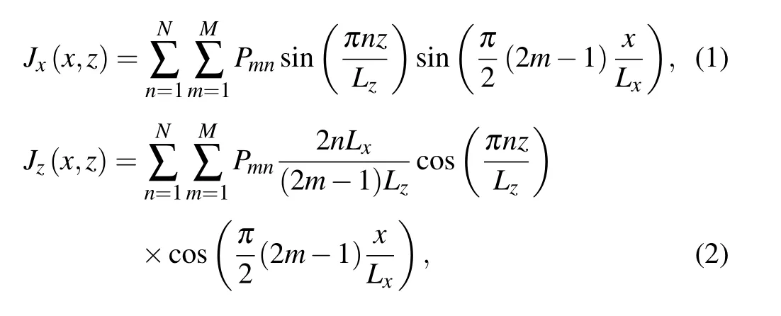
wherePmnis a series of unknown Fourier coefficients with different orders，which are limited by the integral numbersNandM.

By using the Bio–Savart law，thez-component of the magnetic field in the target region produced by the bi-planar coil can be expressed as

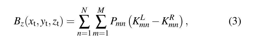
where

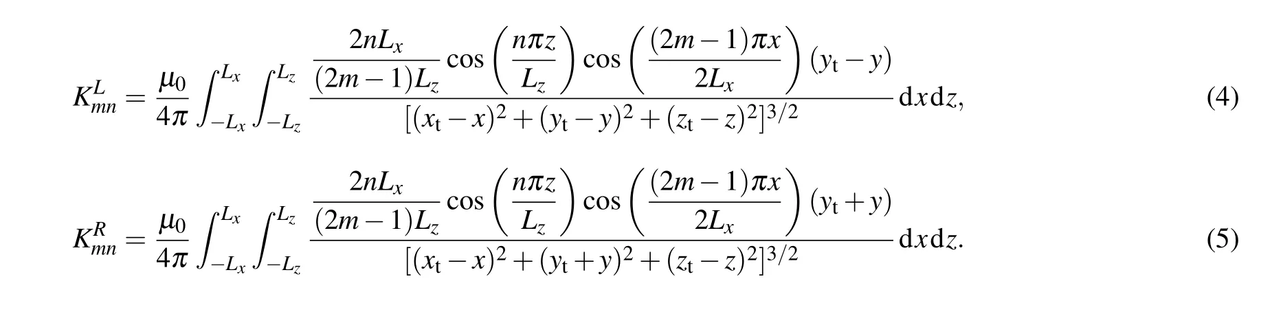
Here，μ0is the magnetic permeability of vacuum，and(x，y，z)，(xt，yt，zt) are the coordinates of the source point and the target point， respectively. Theoretically， thez-component of the magnetic field should be set as a constant，Btarget， in order to keep the magnetic field uniform in the target region， and this relationship can be written as

Note that the current density can be obtained ifPmnare successfully solved here. However，it turns out to be a Fredholm integral equation of the first kind after substituting Eqs. (3)–(5) into Eq. (6). Generally， an objective function together with a penalty item based on the Tikhonov regularization method can be constructed to handle this problem.[12]After setting the magnetic field value at NUM selected target points，Btarget，1=Btarget，2=···=Btarget，NUM，the objective functionFcan be given as

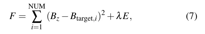
Here，Erepresents the dissipated power， which restrains the length of wires on the coil plane，and hence reduces the complexity of the designed coil.[13]λis a weight factor which should be carefully determined. Given the resistivity and the thickness of the wire，δandt， respectively， the dissipated powerEcan be expressed as

ThenPmncan be obtained by requiring the derivative of the objective function to be zero

According to the target field method， the coil winding patterns are transformed from the contours of the stream functionS(x，z).[14]And the stream function is related with the solved current density and can be expressed as

Finally， based on the maximum and minimum values of the stream function， i.e.，SmaxandSmin， and the pre-determined coil turnsNc， the winding patterns can be visualized by a set of contours which are defined by

For this paper，considering the space limit of our MCG system in the thin MSR，the side length of the bi-planar coil is set as 2Lx=2Ly=1 m， and the distance 2ais set to be 1 m. The side length of the cubic target regionbis set to be 0.3 m，and a total number of NUM=729 target points are selected in this region. Thez-component of the magnetic field in these points are all set to be 1 nT.The integral numbersMandNare both chosen to be 6 after several numerical calculations.The weight factorλis optimized to be 2×10-14viaL-curve criterion.[15]Then the coil winding patterns can be calculated and drawn by the Matlab platform，and the final design result is shown in Fig.1(b). Specially，the solid red and black lines represent the driven current running clockwise and anticlockwise.

Fig.1. (a)The schematic diagram for the design theory of bi-planar coil. (b)The final structure of the bi-planar coil used for residual field compensation.

After importing the coordinates of the obtained coil winding patterns into the COMSOL platform，we can simulate and verify the magnetic performance of this bi-planar coil based on the finite element method. As shown in Fig. 2， the magnetic uniformity error map is used to represent the magnetic distribution characteristics. These three maps exhibit a maximum uniformity error of 50%onXOY，XOZ，andYOZplanes with a side length of 1 m. Whereas in the target region， the auxiliary contours show a magnetic uniformity error less than 0.5%can be provided by this bi-planar coil. This result is satisfying not only because the target region is large enough to cover the whole human thoracic area，but also because the magnetic uniformity in this region is high enough to create a near-zero field area after compensation.

Fig. 2. Magnetic uniformity error maps on (a) XOY plane， (b) XOZ plane，and(c)YOZ plane.

2.2. PID controller

As the residual field is always time-varying inside the thin MSR， the compensation current running in the bi-planar coil should change dynamically in order to keep the field in the target region constantly near zero. To achieve this，a classical PID controller，[16]which is based on the feedback mechanism tracking the real environment， is integrated into the compensation system. The PID theory is usually described by the following mathematical expression:

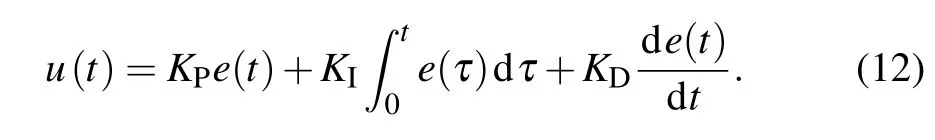
Here，u(t) denotes the control signal which is generated by the PID controller， ande(t)represents the deviation error between the desired result and the measured state. The first part of Eq.(12)is called P-term，which can immediately reduce the errore(t)through proportional response once the deviation occurs. The second part， I-term， is used to eliminate the steady state error through deviation accumulation. And the third part D-term is able to foresee the trend of deviation change and thus produce advanced control.KP，KI， andKDare the proportional， integral， and derivative gains， respectively， whose values should be well tuned to ensure the effectiveness of the P-，I-，and D-term.

Figure 3 shows the schematic diagram of our compensation system based on the PID controller.First of all，in order to obtain a near-zero magnetic field，the set value of this system should be defined to 0 pT. A reference SQUID magnetometer is used here to monitor whether the residual field reaches this set value. The output of the referenceBoutis amplified by the readout electronics and sampled by an analog-to-digital converter(ADC).The output of ADC feeds the difference between the set value and the current measured field into the PID controller， whose output is transformed to a compensation voltageVCOMPvia a digital-to-analog converter (DAC).AndVCOMPcan directly affect the compensation currentICOMPrunning in the bi-planar coil through a voltage-controlled current source. When the residual field after compensation is smaller than the set value，ICOMPshould immediately decrease according to the feedback strategy and the decreased current is strictly controlled by the PID-controller. In contrast，when the compensated field is larger than the set value，the current in the bi-planar coil can also automatically increase after conducting the PID calculation.

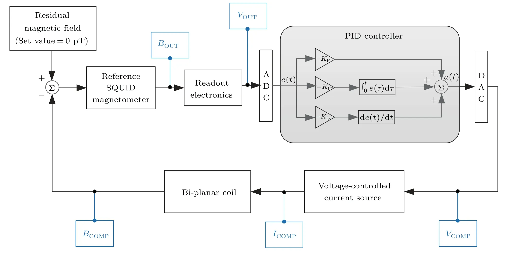
Fig.3. Schematic diagram of the close-loop of the PID-based compensation system.

2.3. System setup

Two SQUID magnetometers， both based on weakly damped Josephson junctions with a large Stewart–McCumber parameter，[17，18]are served as sensing magnetometer and reference magnetometer in our compensation system. As shown in Fig. 4， the sensing magnetometer with a size of 10 mm×10 mm has an intrinsic noise of 4.5 fT/(Hz1/2)，and the reference magnetometer whose size is 5 mm×5 mm has an intrinsic noise of 8 fT/(Hz1/2). Specially，the magnetic field noise of these two magnetometers at 1 Hz are 12 fT/(Hz1/2) and 21 fT/(Hz1/2)， respectively. In general， the sensing magnetometer is arranged at the bottom of the Dewar (see Fig. 5).And the reference magnetometer is placed above the sensing magnetometer coaxially with a distance of 7 cm， which refers to the baseline of a hardware gradiometer we optimized before.[19]Moreover， this thin MSR is manufactured by two layers of permalloy plates and one layer of Al. The thickness of each permalloy plate is 1.75 mm and these two plates are separated by a 100 mm distance. The Al layer，put in the middle of two permalloy plates， is 12 mm thick. The shielding factor of this thin MSR is larger than 40 dB at 1 Hz.[20]

After printing the designed winding patterns on two wooden boards， the bi-planar coil can be fabricated by gluing copper wires on each board. Note that the distance between two boards is 1 m， forming an open space which is large enough to contain a Dewar and a patient. And the Dewar should be carefully arranged to ensure two SQUID magnetometers are located in the high-uniformity target region.Both two SQUID magnetometers can be adjusted to optimal working points via the control units，which are put outside the MSR to avoid additional disturbance.The ADC(NI-9218)and DAC(NI-9260)， integrated in a NI CompactDAQ system， are two independent I/O modules operating at 16-bit resolution. In order to tune three PID gains conveniently，the PID controller is embedded in a Labview platform which can be connected to the NI CompactDAQ via a USB interface. The current source(Thorlabs， LDC200CV)provides compensation current ranging from-20 mA to 20 mA. As the coil constant of the biplanar coil is measured to be 0.4 nT/mA， the compensation ability of this system can reach to±8 nT，which is surely sufficient to cover the amplitude range of the residual field in this thin MSR.

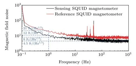
Fig. 4. Magnetic field noises of the sensing magnetometer and reference magnetometer.

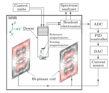
Fig.5. Schematic diagram of the compensation system.

3. Measurement and discussion

After the SQUID magnetometers are immersed into the liquid Helium and tuned to the flux-locked loop mode，the output of the reference magnetometer which carries the residual field information is amplified by the readout electronics and digitalized by the ADC.By using the Ziegler–Nichols method，three PID gains，i.e.，KP，KI，andKD，are fixed as 0.75，0.003，and 0.001 in this case，respectively. Here，the sensing magnetometer acts as a monitor to exhibit the residual field before and after magnetic compensation.

As shown in Fig.6，the outputs of the sensing and reference SQUID magnetometer before compensation，which represent the original residual field in the thin MSR， are firstly measured in time domain. The measurements are conducted during daytime(12:00 am)and last for 30 s. Obviously，these two outputs are well in coincidence with each other， indicating a DC component of 2.8 nT and a fluctuation of 0.8 nT in the residual field alongz-direction. Then， the compensation system is open and the outputs of the magnetometers are recorded in the same way after several seconds，which is spent to track the change of the residual field and adjust the compensation current in the bi-planar coil. The DC component can be suppressed to 0 pT after compensation，but the magnetic fluctuation with an amplitude about 4 pT still exists. It can be assumed that the tracking speed of the reference magnetometer，the digitalized efficiency of the ADC and the calculation accuracy of the PID controller result in this remained fluctuation.And the fluctuation difference from the outputs of two magnetometers can be explained by the position difference between them.Nevertheless，this magnetic fluctuation is acceptable because the MCG signal is 10–20 times larger than it.

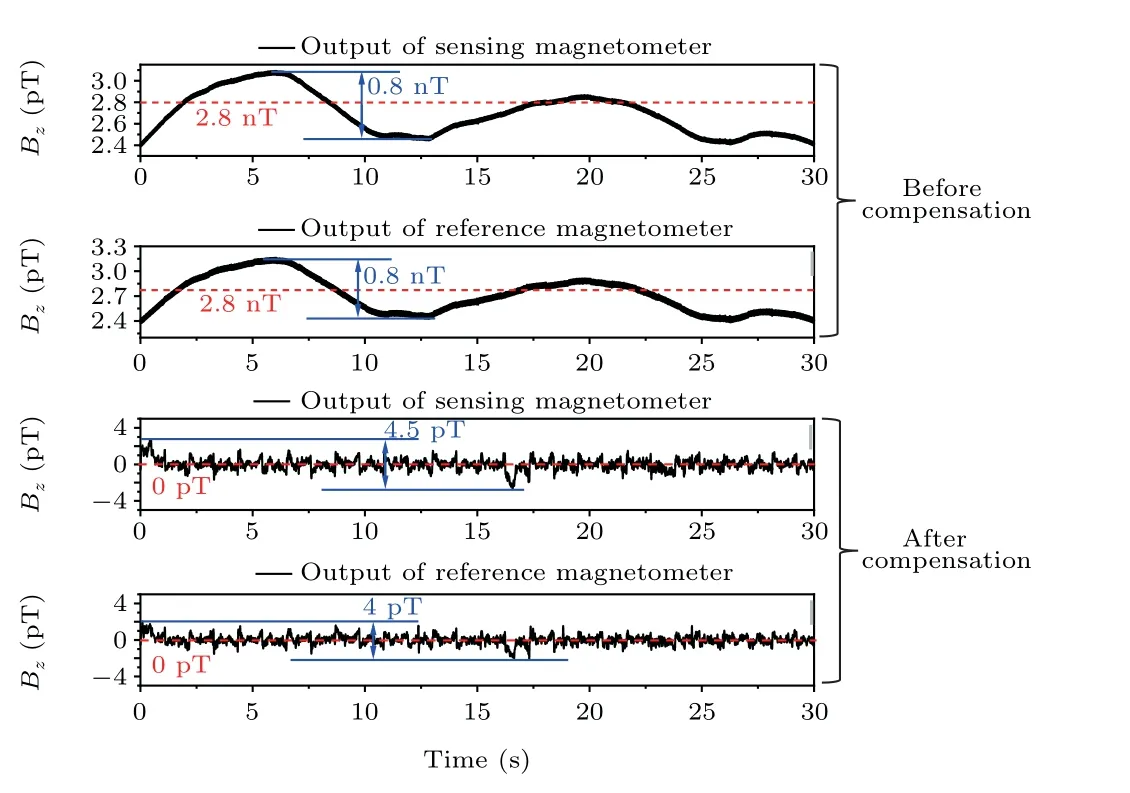
Fig. 6. Residual field detected by the sensing and reference SQUID magnetometer before and after compensation in time domain. The measurement time is 30 s.

The compared results can be further analyzed in frequency domain， as shown in Fig. 7. The white noises of the sensing magnetometer before and after compensation are both 11 fT/(Hz1/2)，about 6.5 fT/(Hz1/2)higher than the intrinsic noise because of the electronic devices used in this system. At 1 Hz，the amplitude of the magnetic noise is 2000 fT/(Hz1/2)before compensation and 200 fT/(Hz1/2)after compensation，exhibiting a noise suppression ratio (NSR) of 20 dB. Specially， the magnetic field noise around 8 Hz with an amplitude of 1000 fT/(Hz1/2) can be effectively suppressed to a normal level with a NSR of 22 dB.And the power-line interference，whose initial amplitude is 800 fT/(Hz1/2)，can also be restrained by this compensation system with a NSR of 26 dB.It is obvious that this compensation system shows an excellent suppression performance in the low frequency range from 0.1 Hz to 50 Hz. As can be seen in the inset， the compensation results of the reference magnetometer are similar with the sensing magnetometer’s， indicating that the residual field can be well compensated in the pre-defined target region.

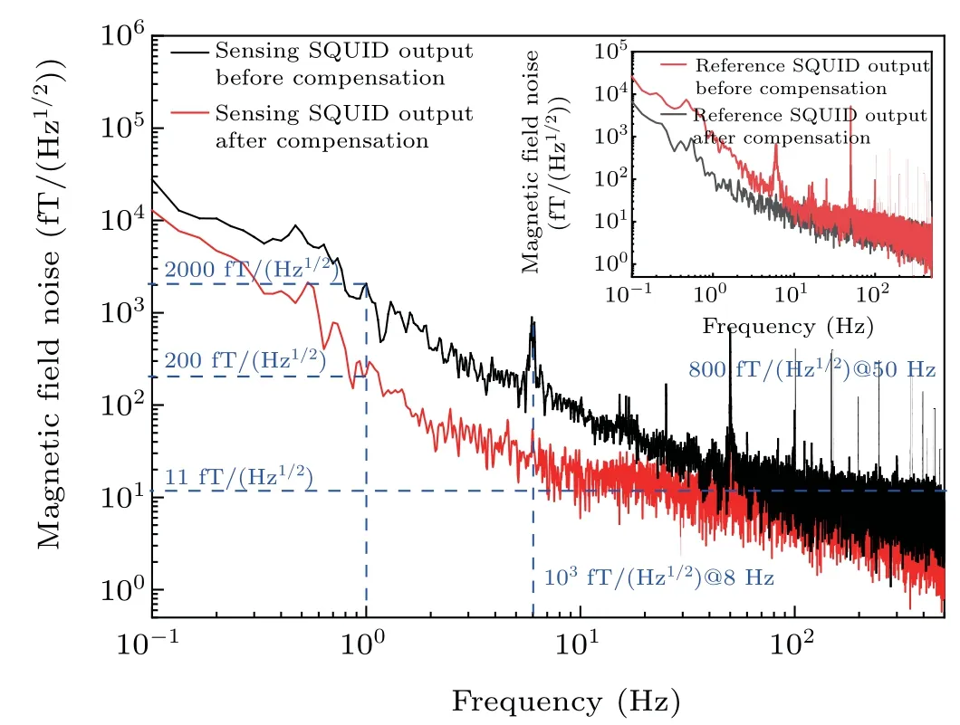
Fig. 7. Residual field from the sensing magnetometer in frequency domain before and after compensation. The inset shows the results of the reference magnetometer.

4. Conclusion

We have introduced a residual field compensation system inside a thin MSR based on a kind of bi-planar coil. The design theory of the bi-planar coil， derived from the target-field theory and the Tikhonov regularization method，has been discussed in detail. The performance of this coil has been well simulated after obtaining the winding patterns via the stream function. Then a classical PID controller has been utilized to control the compensation current in the bi-planar coil， based on the time-varying residual field information provided by a reference SQUID magnetometer. By using this compensation system，the DC component and the fluctuation of the residual field can be restrained to 0 pT and 4 pT，respectively. Also，it turns out that the NSR of the compensation system can reach above 20 dB in the low-frequency range，typically from 0.1 Hz to 50 Hz. Besides the excellent compensation performance，this compensation system can form an open operating space which is convenient for MCG measurement. In the future，this compensation system will be applied in a multichannel MCG system，and even be optimized for other biomagnetic measurement systems.

Acknowledgments

Project supported by the Open Research Fund of Anhui Key Laboratory of Detection Technology and Energy Saving Devices， Anhui Polytechnic University(Grant No. JCKJ2021A03)， the Introduced Talent Research Startup Funds of Anhui Polytechnic University (Grant Nos.2021YQQ006 and 2020YQQ040)，and the National Natural Science Foundation of China(Grant No.62101004).