Parallel optimization of underwater acoustic models: A survey

Zi-jie Zhu(祝子杰) Shu-qing Ma(马树青) Xiao-Qian Zhu(朱小谦) Qiang Lan(蓝强)Sheng-Chun Piao(朴胜春) and Yu-Sheng Cheng(程玉胜)

1College of Computer Science and Technology,National University of Defense Technology,Changsha 410073,China

2College of Meteorology and Oceanography,National University of Defense Technology,Changsha 410073,China

3Acoustic Science and Technology Laboratory,Harbin Engineering University,Harbin 150001,China

4Underwater Acoustics Center,Navy Submarine Academy,Qingdao 266000,China

Keywords: underwater acoustic models, underwater sound propagation, high-performance computing, modeling three-dimensional problems

1. Introduction

Sound waves are currently the only known effective information transmission carriers over long distances in the ocean.Underwater acoustic field data plays an important role in the study of underwater acoustic technologies such as underwater target detection, source localization, and the acoustic exploration of oceanic mineral resources and energy resources. The study of underwater sound propagation is therefore very important.

Underwater acoustic propagation modeling is a common method in computational ocean acoustics for studying underwater acoustic propagation. The prediction accuracy of underwater acoustic propagation loss is affected by the complex marine environment and the accuracy of underwater sound field modeling. There are essentially five types of commonly used models to describe underwater sound:[1]parabolic equation (PE) models, ray models, normal mode (NM) models,wavenumber integration(WI)models(also known as fast field program(FFP)models),and direct finite-difference(FD),finite-element(FE)or boundary-element(BE)solutions of the full wave equation. The first four models all try to solve the Helmholtz equation. The main differences between them lie in the mathematical transformations made before the equation is solved. As shown in Fig.1,they have their own advantages,disadvantages and scope of application. Different acoustic models should be selected for different application scenarios to obtain the optimal solution.

Due to the complexity of the ocean environment and the nonnegligible three-dimensional (3D) effects in most cases,the practical application of underwater acoustic models usually requires very large-scale scientific calculations.This computational demand has grown over the decades as the range of applications has expanded, and thus the computational speed of underwater acoustic propagation models has become more demanding. It has become very difficult to reduce the computation time by improving existing numerical simulation methods of underwater acoustic models. Since the middle of the last century,computers have experienced a period of rapid development and a significant increase in computational speed,from the first high-performance computer parallel vector processor(PVP)in the 1970s,to the early high-performance computer system symmetric multiprocessor (SMP), and then the high-performance computer architecture with massively parallel processing (MPP) using distributed storage structures that emerged in the early 1990s, and cluster systems developed at the same time as MPP. In addition, with the emergence of multi-core processors, a large number of computing units running in parallel can be integrated on a single chip, which greatly improves the computing performance. In many fields of scientific and engineering computing, parallel computing is a common means of speeding up computation. With the rapid development of high-performance computing platforms,scholars in the field of underwater acoustics are committed to applying high-performance computing to the field of underwater acoustic models to improve the accuracy and speed of underwater sound propagation models prediction and meet more research needs.

In this paper,we review the research on high-performance computing of underwater acoustic models since the 1980s and provide an outlook on future work. Figure 2 shows the general developments of underwater acoustic model parallelization over the past four decades. It is worth mentioning that this paper is the first comprehensive literature survey on underwater acoustic propagation model parallel optimization. This paper is organized as follows: Section 2 introduces the development of high performance computing research on parabolic equation models. Section 3 presents contributions to ray model parallel optimization. In Section 4,an overview of normal mode model high performance computing research is presented. Section 5 provides an overview of the development of parallel research on models based on numerical methods for directly solving the wave equation, such as the finite difference method(FDM),finite element method(FEM), and boundary element method (BEM). Section 6 introduces parallelization of other types of underwater acoustic models,such as the BDRM and RMPE hybrid underwater acoustic field computation models, OASES wavenumber integration acoustic propagation model, the parallel dichotomy algorithm for modeling the propagation of acoustic and elastic waves in nonuniform media and the study of parallel methods for solving the sound field propagation in a 3D wedge-shaped seafloor based on the source image method. Finally,Section 7 summarizes and discusses the outlook of the development of high-performance computing for underwater acoustic models.

Fig.1. The advantages and disadvantages of different types of underwater acoustic models.

Fig.2. Developments of underwater acoustic models parallelization.

2. High-performance computing research on parabolic equation models

The parabolic equation method was first introduced into underwater acoustics in the early 1970s by Hardin and Tappertet al.[2]After more than four decades of development,the parabolic equation method has become the most popular wave theory for solving range-dependent underwater sound propagation problems in computational ocean acoustics.

2.1. CPU parallel optimization of the two-dimensional RAM parabolic equation model

The range-dependent acoustic model (RAM) was proposed by Collins[3]in 1993. The RAM is a PE model valid for problems involving very wide propagation angles. It is a very mature and effective PE algorithm currently developed based on the split-step Pad´e method. When calculating with the RAM, there is no direct connection between the sound field calculations at different frequency points,which is ideal for parallel calculations. In 2009,Wang and Peng[4]from the Institute of Acoustics, Chinese Academy of Sciences implemented the fine-grained parallel design of sound field computing using the OpenMP shared-memory model on a multi-core computer for the broadband two-dimensional (2D) parabolic equation RAM.Two years later,Wang[5]carried out message passing interface(MPI)optimization on RAM,which is suitable for coarse-grained computing on a symmetric multiprocessor cluster based on Lujun Wang’s work. In 2015, Brian Dushaw[6]of the Applied Physics Laboratory at the University of Washington released the open source MPIRAM program code on the OALIB website. He first adapted a Matlab version of the RAM proposed by Matt Dzieciuch in Fortran 95, which is not only faster than the Matlab version but also more conducive to handling parallelization-related problems. Since then,he has implemented MPI parallelization and OpenMP parallelization of RAM programs, and experiments have shown that the MPI version of the RAM program is about 4%faster than the OpenMP version on a single CPU.

The key to solving the parabolic equation model is to solve a tridiagonal systems of equations in each range step. In 2015,Sun[7]achieved parallel computing of the fluid PE RAM by solving the tridiagonal linear equations in parallel. There are already several papers related to parallel solutions of tridiagonal linear equation systems.[8–17]Notable among them are the recursive doubling method, the cyclic reduction method and the splitting method. The recursive doubling method was proposed by Stone and Kogge[8,9]in the 1970s for the parallel solution of linear recursive problems, and the LU decomposition of tridiagonal matrices is required before parallel solving. In 1975,Lambiotte and Voigtet al.[15]proposed a cyclic reduction method for solving tridiagonal linear equations in parallel. The basic operation is a primitive transformation that eliminates odd-numbered variables in an even-numbered equation to obtain a system of tridiagonal equations of half size, and then iterating the process. The method was experimentally shown to be most effective on vector computers such as the STAR-100 or CRAY I.A splitting method was first proposed by Wanget al.[14]in 1981. The basic process is to split the matrix into several submatrices, and then the individual submatrices are transformed into unit diagonal arrays through row primitive transformations,which makes the original matrix diagonalized and has good computational stability on parallel computers and vector machines. Subsequently,researchers have improved and extended the splitting method on this basis.[10–13,16,17]For example, Ho and Hohnson[16]improved the method based on the idea of a substructure, reducing the amount of communication. Michielse and Vander Vorst[17]reorganized the computation order of the method to reduce the data transfer.

Sipeng Sun adopted the most widely used splitting method based on a partitioning model,and the split-step Pad´e approximation solution of the fluid parabolic equation is as follows:

Equation(1)can be written in a matrix equation form of the governing equation as follows:

In the second step, the elementdi×kof thei×krow is eliminated (set to 0), and the following calculation is performed for eachi×krow. This step can only be performed serially and can be achieved by adding a Single instruction to the parallel region.

In Eq. (5), vectoryis to be determined, and vectorvis known. MatrixLhas the following form:

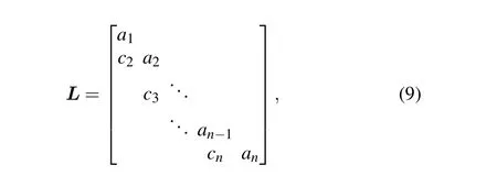
whereai=1,i=1,2,...,n-1,n.

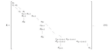
Assuming that the number of processor cores isp, Sun divided matrixLintopsub-matrices of orderk×k(k=n/p),which is shown as follows:

In the first step,c2,ck+2,c2×(k+2),...,c(p-1)×(k+2)of each submatrix are eliminated in parallel,then thec3,ck+3,c2×(k+3),...,c(p-1)×(k+3)are eliminated in parallel,and finallyck,c2k,c3k,...,cnare eliminated in parallel.However,ck+1,c2k+1,...,c(p-1)lk+1 cannot be eliminated in parallel in this step. Therefore, some new elements will be generated during the above elimination process which are recorded asd,and a new matrix in the following form will be obtained:

In the second step,d2k,d3k,...,d(p-1)×kelements of matrix are eliminated sequentially. Finally,ck+1,c2k+1,...,

c(p-1)×k+2;dk+2,d2k+2,...,d(p-1)×k+2;...;d2k,d3k,...,dp×k

elements of matrixLare eliminated in parallel in the third step. The original matrix becomes an identity diagonal matrix after the above three-step elimination process.

Sun conducted numerical simulation experiments with a fluid parabolic equation program, incorporating a parallel tridiagonal linear equation systems algorithm and the original 2D parabolic equation RAM program under a horizontal stratified fluid medium ocean acoustic waveguide. Due to the large amount of extra computation in the splitting method compared to the forward elimination and backward substitution method,the parallel computation time is rather large for a small number of cores (single and dual cores). However, when the number of cores reaches four or eight cores,the acceleration of parallel computing offsets the impact of the extra overhead on the computation time, and the parallel algorithm outperforms the serial algorithm.

2.2. CPU parallel optimization of the 3DWAPE 3D parabolic equation model

Castor and Sturm[18]developed a parallel algorithm based on the 3DWAPE 3D parabolic equation model[19]on a very large parallel computer in 2008. They proposed a parallel strategy with two levels of frequency decomposition and spatial decomposition,in which the frequency decomposition strategy is dedicated to handle broadband signal propagation.The total number of frequencies is divided into multiple frequency groups, where the computation in the uncoupled frequency domain is performed on different processors and all discrete frequencies within the same frequency group are processed sequentially by the same processor. The use of circular redistribution of all discrete frequencies avoids the problem of load imbalance caused by higher frequencies consuming more CPU time than lower frequencies.

Spatial decomposition is applied to acceleration calculations at a single frequency. If the discrete rangernis known,solving the sound field at the next discrete rangern+1requires two successive steps, corresponding to anN×2Dpart and an azimuthal coupling part. The first step is to calculate a total ofnpintermediate sound fieldsu(1)(θ,z),u(2)(θ,z),...,u(np)(θ,z). This step requires the inversion ofM(discrete points in azimuth) algebraic linear systems. The spatial decomposition strategy assigns these inverse operations to different processors,and the results of each processor are assigned to the other processors through interprocessor communication operations in preparation for the azimuthal coupling in the second step. In the second step,u(np+1)(θ,z)is calculated from the last intermediate field obtained in theu(np)(θ,z)first step,which requires the inverse ofN(discrete points in depth) algebraic linear systems of orderM. The parallel strategy is the same as in the first step.

In practice, for broadband 3D-PE calculations, a combination of the above two parallel strategies can be used. The above two parallel strategies(combined form not tested)were verified on several 3D benchmarking cases.Experiments show that a task that takes a day and a half to compute serially on a single processor can be completed in less than an hour using 64 processors (the first parallel strategy is 76% efficient and the second parallel strategy is 50% efficient due to the communication overhead). Considering the computational cost,the serial implementation on a single processor cannot achieve full broadband computing at high frequencies (it takes about an hour of CPU time for a single processor to complete serial 3D calculation at a single frequency of 25 Hz). Nevertheless,after parallel optimization,the broadband computation of 100-Hz pulse can be realized (64 processors perform parallel 3D calculations at 25 Hz in less than 2 minutes).

In addition to benchmark problems, the new parallel 3DWPAE model enables realistic numerical simulations using some classical geophysical models. Castor and Sturm used the parallel 3DWAPE model to study a part of the Mediterranean Sea near the east coast of Corsica and observed a strong change in the modal structure of the 3D field along the east coast,which showing a typical horizontal refraction effect that is different from theN×2Dsolution.

2.3. CPU parallel optimization of FOR3D 3D parabolic equation model

High performance computing platforms were first applied to the study of 3D parabolic equation methods in the 1980s in USA. In 1988, Lee, Saad, and Schultzet al.[20]developed a model (i.e., the Lee–Saad–Schultz (LSS) model) for predicting sound propagation problems in a 3D marine environment based on an implicit implementation of natural alternating directions(ADI).The solution process of the LSS model equations is implemented in the FOR3D program,[21]combining an ordinary differential equation technique, rational function approximation and an implicit finite difference method. The FOR3D calculation process is shown in Fig.3. First,a sound field space is gridded on a cylindrical coordinate systemr–θ–z, and then the sound pressure value on each grid point is solved by starting from a given initial field and advancing outward along the cylindrical radial direction until the sound pressure calculation of the whole sound field region is completed. In the same year,Leeet al.[22]tested the FOR3D program using two state-of-the-art supercomputers: the CRAY X-MP and the Intel iPSC/2. Later in 1994, Leeet al.[23]designed a FOR3D parallel algorithm using the Linda parallel programming language and completed implementation on a BRMD6000/560 cluster workstation.

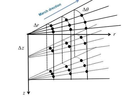
Fig.3. Solutions are marched outward in range by repeatedly solving tridiagonal systems of equations in FOR3D.

In 2015,Sun[24]studied the parallel strategy of anN×2Dapproximation method for FOR3D and the real-time visualization of an underwater 3D sound field. The approximation method is to solve the standard parabolic equation using the split-step FFT algorithm proposed by Hardin and Tappert to obtain the 2D sound field in a certain direction.Such 2D sound fields inNdirections can approximately form the sound field of the whole 3D space. Therefore,they adopted two layers of parallelism. The first layer is the coarse-grained parallelism of the MPI model for the 2D sound field between different azimuths,and different orientation sectors are assigned to different MPI nodes to perform the relevant calculations. The second layer is a fine-grained OpenMP parallel computation within nodes for the FFT algorithm.

In 2017, Xu[25–28]investigated a single-core serial performance optimization method,multi-core multi-threaded parallel computing method and MPI+OpenMP hybrid parallel computing method for FOR3D based on the Tianhe-2 supercomputer[29]and Intel’s second-generation MIC architecture of Xeon Fusion Series KNL processor.[30]On typical multicore processors,the optimized FOR3D model calculation speed can be increased nearly 30 times for single frequency calculations and up to 128 times for broadband sound field calculations.

Sequential optimization on a single core for the FOR3D model includes compiler optimization,the use of high performance libraries and application of vectorization operations.Compiler optimization includes the choice of two different compilers,GNU and Intel,and the choice of different compilation options,-O2,-O3,-ipo,-funroll-all-loops and-parallel.The use of high performance libraries refers to the application of BLAS and LAPACK subroutines in Intel’s Math Kernel Library general mathematical core function to replace the TRID subroutine in the original FOR3D to solve tridiagonal linear equations. The application of vectorization includes the addition of the#pragma ivdep compilation guidance statement for manual vectorization in the“two-step”code for calculating the right-hand side(RHS)and two coefficient matrices and using the AVX512 instruction set on the KNL to replace the default SSE2 instruction set of the compiler.

Before performing FOR3D multi-threaded parallel optimization on multi-core processors, Xu changed the original methods of reading files, writing files and computing processes alternately by decoupling I/O operations and computations from each other. The changed program takes full advantage of the high-bandwidth I/O,laying the foundation for parallel optimization of subsequent computation processes. Using the Intel Vtune hotspot analysis tool, she found that the program hotspots were concentrated in the twostep function,a subfunction of the “two-step” equation (the twostep function of the example calculation took 71%of the total running time). Although there is data correlation between each range step (the calculation of the sound field at distancer+Δrrequires the data of the sound field at distancer),the calculations at the same range,in different azimuths or at different depths are independent. Therefore, the OpenMP model can be used to assign the calculation of the two-layer loop of the RHS of the equation and the depth and azimuth of the coefficient matrices to different threads for parallel computation. As shown in Table 1, the computational power of the Tianhe-2 node is higher than that of the KNL node, but the latter is more suitable for programs with high computational concurrency(for a typical test case,the speedup ratio of FOR3D is 25.77 on the Tianhe-2 and 28.06 on the KNL).

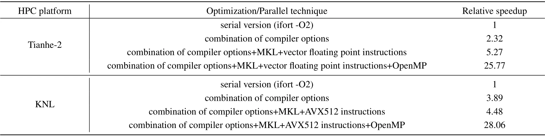
Table 1. Optimization and parallel results of FOR3D on Tianhe-2 and KNL.

For independent calculation between different frequency fields of the broadband 3D sound field of the FOR3D, Xu uses MPI to directly parallel optimize the calculation of each frequency point. In addition, the computation for a single frequency of a process can be realized using the parallel optimization method mentioned above, thus realizing MPI+OpenMP hybrid parallel programming for the FOR3D model. The experimental results showed that the acceleration effect of the Tianhe-2 is better than the KNL when the multiprocess parallel programming mode is used alone. However,when thread parallelism was added,the KNL acceleration effect improved significantly,and the maximum acceleration ratio reached 128.67,which exceeded the acceleration effect of the Tianhe-2 nodes.

2.4. GPU parallel optimization of parabolic equation models

The uathors in Ref. [31] reviewed the implementation of the split-step Fourier parabolic equation model called GPUwave(proposed by Tappertet al.in 1977,[32]and the authors in Ref.[33]provide a detailed implementation)on a GPU proposed by Gunderson before the advent of CUDA, using C++, OpenGL, and OpenGL Shading Languages (GLSL)[34]to program GPU shader elements. The implementation focuses on the discrete sine transform (DST) and fast Fourier transform(FFT)processes. Experimental results showed that GPUwave is three orders of magnitude faster than the Matlabbased stepwise Fourier PE model PEEC,[35]and the model accuracy is comparable to that of the RAM[3]and the wavenumber integration model Ocean Acoustics and Seismic Exploration Synthesis(OASES).[36]

In 2011, Hurskyet al.[37]implemented GPU parallel optimization of the split-step Fourier parabolic model using CUDA.They took advantage of the fact that the PE model is a narrow-band model and that the broadband application of the model requires running multiple frequencies covering the desired frequency band to form the predicted time-domain waveform by inverse FFT synthesis and discovered the potentially parallelizable part.They referred to Ref.[38]to implement the GPU-based part of the tri-diagonal system of equations solution for PE formulation, implemented GPU-based FFT computation based on the CUFFT library[39]provided by CUDA,and reduced the I/O overhead by executing the GPU computation,CPU computation,and data transfer in parallel. Subsequently,they compared the optimized model with the Scooter wave number integration model[40]and the RAM in a Pekeris waveguide and wedge seafloor environment to verify the accuracy and compared the computational performance with the CPU multi-core implementation version based on the FFTW library[41]on three range-dependent modeling cases. It was shown that the GPU version is about ten times faster than the multicore version using OpenMP.

In 2019,Leeet al.[42]developed a 3D parabolic equation model in a Cartesian coordinate system. The model contains the same higher-order cross terms as the 3D-PE models developed by Lin[43]and Sturm.[44]In contrast,Keunhwa Lee’s model first splits the full step-by-step 3D-PE solution into two exponential terms (non-crossover terms) and one exponential term(crossover terms)before approximating each term using the Pade approximation and Taylor expansion. In addition,they improved the computational accuracy of the model by using rational filters for theYandZoperators of the cross terms.In the same year, Leeet al.[45]implemented a GPU version of this 3D-PE model. They discovered potential GPU parallelism by exploiting the feature of each exponential operator being approximated by a Taylor series and the sum form of the Pade approximation,and implemented a matrix multiplication and inversion strategy using the cuSparse library in CUDA/C.The total computational performance of the GPU version was experimentally shown to be improved by a factor of 5 to 10.

3. High-performance computing research on ray models

In the early 1960s, underwater sound field models were mainly developed using ray tracing methods. The earliest research on ray-tracing theory in the field of hydroacoustics dates back to 1919 when Lichte[46]compared measured data and model results in different shallow sea environments.A ray method is a high-frequency approximate solution of the wave equation, and traditional ray theory cannot handle low-frequency problems. However, the BELLHOP model[47]based on Gaussian beam breaks this limitation,especially with better adaptability for both high and low frequencies in a deepsea environment. Although ray models have the problem of less accurate results in the low-frequency environment of shallow seas, they are suitable for situations with high time requirements such as actual combat because of their high computational efficiencies and clear physical images.

3.1. CPU parallel optimization of ray models

The prediction of ray models is generally carried out in two steps: The first step is to solve the trajectory of each ray by solving the set of Eikonal equations. The second step is to calculate the coherent superposition of Gaussian beam effects at the position of the receiving hydrophone as the predicted sound pressure field there. The main difference between the different ray models lies in the different numerical strategies used.

The sound field calculation of the BELLHOP Gaussian ray model is superimposed according to the contributions of different rays,and it is very suitable to allocate computational tasks according to different rays calculations to achieve parallel optimization. The parallel strategy for ray models is generally to divide the workload at the ray level. In 2011, Chen and Peng[48]of the Institute of Acoustics, Chinese Academy of Sciences (CAS) designed a parallel algorithm for BELLHOP using MPI and conducted experiments on a multiprocessor cluster system. In 2019 Zhang and Sun[49]of the CAS,developed a parallelized ray model BellhopMP for the C++version of the BELLHOP propagation model, BELLHOPC,using multithreading techniques. They divided the sound ray angles into multiple intervals, and the main thread computes only the contributions of the beams to the sound field in the first interval. Each of the other threads calculates the sound field of beams in a certain angle interval. Finally, the main thread collects the results of all threads and outputs the results to a file. A certain speedup has been achieved on computers with multi-core processors. The BELLHOP parallel computing method is shown in Fig. 4, whereMrepresents the total number of rays,Nrepresents the total number of parallel nodes andM/Nrepresents the number of rays to be calculated per node.

Fig.4. Parallel computing method of BELLHOP.

In 2013, Xinget al.[50]proposed a parallel algorithm for seeking 3D eigen-rays in an irregular seabed based on OpenMP.The parallelization steps of the algorithm are divided into two major parts. The first step is ray-tracing calculation.Because the computation of each grazing angle is independent of each other, the trajectory of each ray can be computed in parallel according to the step size. In addition, because ray trajectories with adjacent grazing angles are similar and require approximately the same computational effort, they can be classified according to the initial grazing angle to obtain a high computational efficiency. The second step is to calculate the eigen-rays from each group of similar rays in parallel,given that the eigen-ray calculations of these groups are not correlated.They used this model to implement eigen-ray seeking,the computations of ray tracing and transmission time of eigen-rays in parallel (where the maximum number of parallel threads is the number of CPUs of the computing platform)and performed experiments on a quad-core CPU test with a speedup ratio of 3.76.

In 2017, Rog´erioet al.[51]of the SiPLAB proposed a parallel implementation method based on open MPI[52]for TRACEO3D. The TRACEO ray model was proposed by the Signal Processing Laboratory (SiPLAB) of the University of Algarve in 2011.[53,54]It allows the prediction of sound pressure in complex boundary environments. The TRACEO3D ray model is a 3D extension of TRACEO that considers outof-plane propagation. The model algorithm is executed in two steps. The first step is to solve the trajectory of each ray by solving the set of Eikonal equations. The second step is to calculate the coherent superposition of Gaussian beam effects at the position of the receiving hydrophone as the predicted sound pressure field there. This work divides the workload at the ray level,while adjacent rays are executed in different processes to avoid acquiring a larger number of relatively more time-consuming rays by the same process(rays with adjacent emission angles have similar trajectories and thus have similar execution times). They evaluated the accuracy and performance of the parallel implementation of the model by conducting a tank scale environment. The experimental results suggested that the parallel implementation of TRACEO3D based on open MPI is 12 times faster than the serial version, and 5 times faster compared to other models (BELLHOP3D (the three-dimensional extension of the BELLHOP ray model)[55]and KRAKEN(a model based on normal mode theory).[56]

When dealing with adjacent rays, Chuanxi Xing and Rog´erio both took into account the fact that adjacent rays have similar grazing angles and therefore require approximately the same computational efforts. From the perspective of workload balancing among parallel processes(or threads),both methods allocate the subsequent computations of adjacent rays to different processes,thus avoiding the problem of load imbalance caused by the relatively more time-consuming rays only acquired by several processes(or threads),which may results in a decrease in computational efficiency.

3.2. GPU parallel optimization of ray models

In 2006, Haugeh˚atveit[57]used a ray model called PlaneRay[58]developed by Hovemet al. of the Norwegian University of Science and Technology,implementing the first calculation part of the model on a GPU, that is, the initial ray tracing without acoustic intensity and beam displacement.They set a ray to a pixel, and the size of the pixel grid as the number of rays.The PlaneRay model computes the sound field with multiple iterations,treating the GPU as a stream processor, and each iteration performed on the stream generates a frame, with the number of frames created determined by the pixel grid size. Each frame is stored in a frame buffer and used as input to the next iteration.

He used GLUT (OpenGL’s program library) for the initial setup, copying the sound speed profile and other initial settings (such as source depth, bottom depth, receiver depth,and other information)to the GPU’s textures via arrays on the CPU(with the help of Shallows,this can be done with just one statement) as inputs to the Math Shader (a small program in the main program that is used for mathematical calculations).The values in the texture are stored as quaternion vectors(i.e.,four different values sent from a texture to each pixel), and both the frame buffer and the texture are forms of data storage on the GPU, called render targets. The data in the on-screen frame buffer is passed to the screen through the Render Shader(a small program in the main program that is used for rendering), which is used to display the ray paths on the screen. In addition, since each calculation overwrites the frame buffer in the GPU, it is necessary to store all results in the frame buffer on the CPU by reading them back asynchronously.Olav Haugeh˚atveit conducted experimental tests on a computational grid of 410×410 and compared to the Matlab version of the PlaneRay model,the GPU version of the PlaneRay model performed almost 200 times better when computing up to 4×104rays.

In addition to the above CPU-based parallel optimization for the TRACEO3D model, the SiPLAB at Algarve University also performed parallel GPU-based optimization for the cTraceo ray-tracing model(2D)and the TRACEO3D model it developed. The comparison of three versions of parallel optimized Traceo ray models is shown in Table 2.

Table 2. Comparison of optimized versions of Traceo ray models.

In 2013, Emanuel Ey[59]of the SiPLAB addressed the adaptation of the cTraceo model from a single-threaded CPU implementation to a GPU-based implementation based on the OpenCL programming framework.[60]He created a thread for each emitted ray. Specifically,a kernel is first launched to simultaneously solve the Eikonal equations for all rays. The data generated by the Eikonal solver is then passed to a transport equation solver,which calculates the ray amplitudes along each ray in the form of one thread for each ray. Finally, the threads are started in the same form,and a simple dichotomy is used to find the ray coordinate index nearest to each hydrophone for a ray path consisting of a series of points in space. Thereafter, depending on the output options, the calculation of the arrival pattern and the sound pressure is implemented. Subsequent experimental tests showed that the model’s runtime remains approximately constant when the number of computed rays is less than the number of cores of the GPU(512). However, when the number of rays is higher than the number of cores of the GPU,the runtime keeps growing at the same rate as the number of rays. In addition, the startup and initialization times generated by the OpenCL programming framework reduce the performance gain for simple waveguides and low ray counts, making it more suitable for modeling calculations at high ray counts.

SiPLAB researchers implemented the GPU parallel optimization of TRACEO3D using a CUDA programming model[61]based on an NIVIDIA GPU.[62]Before the parallel implementation,they first optimized memory organization.When processing thousands of rays in parallel, if the ray trajectory information are all stored in memory,the memory will soon be in an overflow state. To avoid this problem, only the values calculated for each ray segment regarding ray path and amplitude are stored in memory,and only three data segments at timest,t-1, andt-2 are stored in memory, greatly reducing the amount of stored data. In addition,they considered the storage locations for various types of data based on their size and frequency of access(e.g.,the sound velocity data was placed in shared memory because it needs to be accessed frequently during ray-trajectory calculations; however, the data on environmental boundaries were moved to global memory because of the large amount of data for the 3D waveguide case). It has been proven that the model can be computed approximately 170 times faster than the serial implementation through improvements in parallelism and numerical modeling.

3.3. Research progress of ray tracing technologies on a GPU

In recent years, there have been many advances on ray tracing technology on a GPU. In 2009, Aila and Laine[63]proposed including replacing terminated rays and using work queues to improve the single instruction,multiple data(SIMD)efficiency of ray traversals on GPUs. In 2010, Aila and Karras[64]proposed a GPU architecture for improving ray tracing performance that supports a technique called Work compression: if more than half of the rays in a warp have terminated,then the unterminated rays are re-queued to the work pool. A special hardware structure is needed to support this frequent queue operation. In addition, they propose an optimization to improve performance: if a queue is bound to another processor,rays in that queue do not need to be requeued in memory but can be transferred directly to the bound processor. In 2018,Lieret al.[65]studied ray traversal on the Pascal architecture(the predecessor of the Turing architecture)based on the work of Aila and Laine and proposed new techniques such as intersection sorting to improve performance.

In 2019,Joacim St˚alberg and Mattias Ulmstedt,[66]based on previous work experience, studied the simulation of underwater sound propagation in two-dimensional space based on ray tracing method on a GPU using NVIDIA’s OptiX[67]ray tracing engine, and named their implementation the OptiX Sound Propagator (OXSP). Their work realized various degrees of parallelization in ray classification, ray sorting,eigen-ray interpolation, graphics and signal generation, fast Fourier transform, and point-by-point multiplication of frequency functions. At the same time, they also introduced RT kernels for the acceleration of certain calculations in ray tracing. RT kernels are very efficient for bounding volume hierarchy(BVH)traversal and testing ray-primitive intersections.Experimental results showed that the OXSP can achieve up to 310 times speedup using an NVIDIA RTX 2060 graphics card compared to the CPU-based Fortran implementation of BELLHOP.

4. High-performance computing research on normal mode models

The normal mode method is suitable for a problem calculating long-range acoustic fields at low frequencies in the deep sea. The first widely cited literature on the normal mode method in underwater acoustics is the simple two-layer ocean model theory proposed by Pekeris in 1948.[68]However, the early normal wave models could only propagate in horizontally stratified oceans, and thus could only solve very limited practical problems. The coupled-mode approach was proposed in the 1960s,[69,70]and subsequently developed by Rutherford[71]and Evans.[72]The method takes into account the coupling between each different-order mode and is applicable to all frequencies; therefore, it can handle the twodimensional acoustic propagation problem with horizontal variation and high computational accuracy. Since the biggest drawback of coupled simple positive wave theory is the large computational effort,some researchers have studied the parallel optimization of coupled-mode methods in recent years.

4.1. CPU parallel optimization of the KRAKEN normal model

Kraken models solved the numerical instabilities of early normal models for certain type of sound-speed profiles and the inability to calculate a complete set of ocean modes. In 2008, Liu[73]realized distributed parallel computing for the single-frequency long-range sound propagation KRAKENC mode[56]based on network-connected PCs using Windows Sockets. In the KRAKENC model,the normal mode coupling coefficient matrix from the sound source to the receiver contains the important information of the sound field. The matrix is divided intoQsegments along the horizontal direction of the sound propagation, and the number of normal waves isN, then there areN×Qcalculation subtasks. The computations between the subtasks are independent,which is suitable for parallelization. The parallel system was implemented under the Windows operating system using Visual C++network programming,[74]which is not conducive to practical applications because the achievable parallelism is very limited. In addition,Li[75]also parallelized the broadband sound field calculation of KRAKEN using the OpenMP programming model taking advantage of the fact that each frequency calculation does not affect the others.

4.2. CPU parallel optimization of the WKBZ normal mode model

The most difficult part of normal mode models is the calculatoin of eigenvalues. There are many methods for solving the eigenvalues, and each of these methods has its own advantages and disadvantages. The conventional normal mode models like KRAKEN are difficult to calculate the eigenvalues and eigenfunctions,and therefore cannot be applied to broadband and pulse propagation applications. The WKBZ mode approach[76]can realize accurate prediction of a sound field in a deep sea environment and is an effective means to understand the law of underwater acoustic propagation in deep-sea environments. The WKBZ (WKB refers to Wentzel–Kramers–Brillouin, and Z refers to Zhang Renhe, from the Institute of Acoustics,CAS,who improved the shortcoming of the divergence of the WKZ approximation at the reversal point) approximation is one of the approximate methods to find the roots of the characteristic equation in normal mode computation. The WKBZ mode approach[76]can realize accurate prediction of a sound field in a deep sea environment and is an effective means to understand the law of underwater acoustic propagation in deep-sea environments. In recent years,scholars have studied the parallel optimization algorithm of the WKBZ normal wave model based on a high-performance computing platform and achieved good performance results.

How to improve the computation speed of eigenvalues is the key point of parallel optimization of normal mode models. In 2006, Daet al.[77]implemented a parallel algorithm for eigenvalue,eigenfunction and propagation loss calculation of the WKBZ normal mode model based on an MPI parallel programming model in a PC cluster-based experimental environment. In the process of solving the eigenvalues, there is no correlation between the computation of the eigenvalues of each simple positive wave, and thus parallelization can be achieved naturally.As for the calculation of the eigenfunction,the number of eigenvalues is decomposed by blocks,and each continuous segment is assigned to the corresponding process for calculation. The size of each segment is basically the same to ensure load balancing between processes.The design of this algorithm needs to consider the relationship between the total amount of computation and the number of processes because the parallel efficiency decreases due to the increase of interprocess communication time when the computational load is small at low frequency.

The above-mentioned parallel work of WKBZ mode method was carried out on mutiple Linux-based PCs. In contrast, In 2010, Liuet al. investigated multicore and cluster parallelization methods for WKBZ mode computation[78,79]in 2010. The central idea of optimization is to first use the MPI model to coarse-grain divide the computational tasks into subtasks on different nodes,and then use the OpenMP model to continue the fine-grained division of these subtasks on the multicore system at each node. Experiments show that the acceleration ratio of the multicore system is about 90% of the parallelism, while the acceleration ratio on the cluster is about 40%–60% of the number of processor cores. In addition, by comparing the price/performance ratio (acceleration value divided by the total price of processors in the system)of the two systems,the computational price/performance ratio of the multicore system is better than that of the cluster system.The parallel optimization algorithm for the 2D WKBZ normal mode model was also studied by Fanet al.[80]in 2020 based on the MPI+OpenMP programming model and the basic idea was the same as Liuet al.

5. High-performance computing research on underwater acoustic models based on direct discretization methods

For a two-way wave equation in a heterogeneous fluid elastic environment with complex structure, it is necessary to solve using numerical methods based on some direct discretization of the governing equation. At present, numerical methods of this type are mainly divided into three categories:finite difference methods(FDMs),finite element methods (FEMs) and boundary element methods (BEMs).[1]Although these methods have high computational accuracy,they are computationally intensive and slow because the discrete solution needs to be able to represent the actual spatial and temporal variation of the sound field. Therefore, there is a great need for parallel optimization.

5.1. Parallel optimization of underwater acoustic models based on finite difference methods

In 2013, Joseet al.[81]studied different parallelization methods of the finite-difference time-domain (FDTD) for indoor 3D acoustic modeling based on a GPU platform. He adopted a CUDA programming model to achieve GPU parallel optimization considering its flexibility and developer friendliness. The CUDA model benefits from its hierarchical structure to deal with 2D data with great flexibility. However,since the grid can only be two-dimensional,he considered the tiling and slicing methods to deal with 3D data problems. For the CUDA model, a GPU is considered a device containing a set of memory and a set of independent streaming multiprocessors(SMs).The tiling method allocates a thread for each data point and keeps the streaming multiprocessor busy. This method is divided into 1D tiling and 2D tiling, which involve index transformation in the process of dimensionality reduction.The 1D Tiling method is preferred because of the low computational effort involved in index transformation. Depending on where the data is stored, it is divided into two methods: tiled global and tiled shared. The former requires direct access to the global memory, which is time-consuming. For the latter,the model data is stored in the shared memory, and only the data of the upper and lower nodes need to be read from the global memory.

The second approach to handle 3D data is called slicing, which uses 2D thread blocks and slices the entire volume along thezdimension of the thread blocks(called threadfronts). This thread block scans the entire volume along thez-dimension at each time step,where each thread processes a given column of nodes. For this data processing method,texture memory can be used for optimization. The cache space of the texture memory is optimized for the locality of 2D space,and is actually used by texture references to point to a specific spatial structure in global memory and define which part of that space is fetched in which way. In addition,it is necessary to divide the 3D data into multiple subvolumes and treat the whole 3D data as a stack in the form of a stack. The width and height of the 2D texture reference are obtained according to the three cases where the subvolume is located at the bottom,middle and top of the stack.

Therefore,according to the two 3D data processing methods and the use of the used memory subsystem provided by the GPU, six different implementations were proposed, namely tiled shared,tiled global,naive,shared texture fetching,shared global and pure texture fetching. Performance tests were conducted using both Tesla and Fermi architectures, and it was found that for the Tesla architecture,pure texture fetching has the best results,while for the Fermi architecture,shared global achieves the best performance for single-or double-precision floating-point model data. Furthermore,the GPU-parallel optimized model is two orders of magnitude faster than the sequential implementation.

In 2015, Hern´andezet al.[82]studied a 3D finite difference implementation of the sound diffusion equation, which is a common tool in room acoustic modeling, using a massively parallel architecture and evaluated the latest generation of NVIDIA and Intel architectures. They first rewrote the original single threaded version of Matlab in the C language,then developed two different parallel implementations: (i)the C/OpenMP version with vectorization for Intel Xeon Phi architecture[83](with SIMD support) and (ii) the CUDA[84]parallel optimized implementation based on an NVIDIA GPU architecture.

The Intel Xeon Phi architecture has a vector processing unit (VPU) that implements vectorization using the #pragma simd pragma statement (forced vectorization) in OpenMP4.0 and aligning data (which includes aligning base pointers when allocating space for data, using themm malloc() and mmfree() instructions to ensure that the starting index of each vectorized loop is aligned, and using-assemptionaligned(-matix,64) for dynamically allocated arrays instruction). For the CUDA implementation based on the NVIDIA GPU architecture,they employ a tiling technique that exploits data locality through shared memory. Specifcially, the entire volume is divided into multiple 2D blocks with initial values,each block corresponds to coordinates (x,y), and the size of each block isz.Each CUDA thread corresponds to a grid point(x,y,z), and threads in the same 2D block share information by sharing memory and registers,thus making full use of data locality.

Subsequently,As shown in Table 3,the authors evaluated the performance and energy consumption of 3D-FD for different indoor resolutions (i.e., 128×128×128 (32 megabytes),256×256×256 (256 megabytes), 384×384×384 (864 megabytes),and 512×512×512(2048 megabytes))based on an Intel Xeon,Intel Xeon Phi,and NVIDIA GPU[85](Kepler(TeslaK40c), and Maxwell GPU (980GTX)) platforms, separately. Experiments show that the GPU significantly outperforms the Xeon Phi and CPU implementations for all resolutions. NVIDIA Maxwell GPUs provide the most efficient acceleration. When considering performance-oriented metrics such as EDP,NVIDIA’s high-end GPUs(E3slaK40c and 980GTX)are more suitable for 3D-FD calculations(at an indoor resolution of 512×512×512 (2048 megabytes), the NVIDIA GPU delivers 5 times faster performance than the Intel Xeon Phi and 31 times faster than the Intel Xeon CPU).In addition, the separate memory interface/hierarchy (GDDR5)for the Intel Xeon Phi and NVIDIA GPUs addresses memory space constraints when problem sizes become large.

Table 3. Summary of the empirical results.

In 2016, Longet al.[86]proposed a second-order finitedifference underwater acoustic model for simulating the sound propagation problem in a 3D coastal environment. When the complex sparse matrix is large and the matrix equations are difficult to solve in the case of high frequencies and large area ranges,he used the complex shifted Laplacian preconditioner(CSLP) method[87]and the biconjugate gradient stabilized(BiCGStab) Krylov subspace method[88,89]or GMRES[90]to iteratively solve the matrix system. For numerical simulation experiments of a coastal wedge case, he used a parallel implementation of the BiCGStab and GMRES methods in the PETSc library[91]to perform simulations on 25 computing nodes(each with 24 cores)of a clustered system,reducing the model run-time,originally measured in days,to approximately 4 hours.

In 2021, Liuet al.[92]of the School of Meteorology and Oceanography,National University of Defense and Technology proposed Computational Ocean Acoustics–Helmholtz(COACH), a 3D finite-difference model with formal fourthorder accuracy for the Helmholtz equation in ocean acoustics.The model solves a system of linear equations using a parallel matrix-free geometric multigrid preconditioned biconjugate gradient stabilized iteration method,and the parallel code is run and tested on the Tianhe-2 supercomputer.

The decomposition strategy for the parallel solution of the 3D sound field of COACH is shown in Fig. 5.[92]The entire 3D sound field is decomposed intoMx,My,Mzgrid blocks in three dimensions,each block containingmx×my×mzgrid cells(the values ofmx,my,mzneed to satisfy the integer powers of two for successive multiple grid coarsening), and each block corresponds to an MPI process for computation. For the asymmetric matrix system in the COACH model, Liu Weiet al.used the BiCGStab method for the solution considering the memory cost. The pressure at the grid points near the interior boundaries must be exchanged with adjacent blocks before the stencil computations of the formal fourth order FD schemes can be performed within each outer iteration of the BiCGStab method. This is done using communications between the corresponding MPI processes. In addition, the matrix-free geometric multigrid preconditioner is used to solve the precondition equations in each outer iteration of the BiCGStab technique. The smoother(symmetric Gauss–Seidel in the study),restriction,and interpolation operations on each grid level are carried out inside the grid block in the multigrid preconditioning technique,however they require communicating with one grid layer near the inner boundaries.

Fig.5. Decomposition strategy for the parallel solution of 3D sound field of COACH[92]@Copyright 2021 JASA.

To test COACH,four 3D topographic benchmark acoustic cases, a wedge waveguide, Gaussian canyon, conical seamount, and corrugated seabed, were simulated, with the wedge waveguide case having the most grid points (33.15×109), operating in parallel with 988 central processing unit cores.

5.2. Parallel optimization of underwater acoustic models based on finite element methods

Finite element methods (FEMS), like finite difference methods(FDMs),are numerical methods based on direct discretization of the governing equations and thus also have significant computational and storage costs. Although an FEM can work more easily on curved seabeds,until now 3D FEMs have only been suitable for acoustic simulations on a relatively small scale because they must store additional connectivity tables listing the points in the vicinity of each cell,and thus limiting the practical problems that can be solved.In the last three decades,scholars have conducted extensive research on parallel optimization problems for FEMs.

In the mid-1990s,Kazuo Kashiyama,Katsuyaet al.[93–95]used parallel FEMs to study large-scale tidal currents and storm surges and used the methods to study the actual problem of surge in Tokyo Bay. In 2000, Caiet al.[96]implemented parallel computation of 3D nonlinear sound field simulation on a Linux cluster system. In 2003,Brettet al.[97]performed parallel computation of the flow field for a simulated rectangular shallow water basin(4000-m long, 2500-m wide,and 6-m deep) using an implicit finite volume shallow water model based on a parallel Boewulf cluster system. In 2004,Asavanant,Lursinsapet al.[98]conducted a parallel numerical simulation of the dam failure problem using a finite volume approach.

In 2002, Cecchi and Pirozzi[99]implemented a shallow water finite element model in parallel on a multi-instruction multi-data distributed storage multiprocessor using the MPI programming model for simulating tidal motion in a Venetian lagoon. The biggest problem of the model was how to achieve load balancing in a non-uniform computational domain. In fact,the problem of unstructured meshing has been a very important area of research. The most straightforward approach is the recursive coordinate bisection(RCB)algorithm,but the biggest problem of this algorithm is that it does not use any connectivity information between the sub-regions and thus creates a high communication requirement. Another method,called recursive graph bisection (RGB), divides subdomains based on the two vertices that are most separated by the graph distance (the minimum number of edges that must pass between two vertices). There is also a better but more expensive technique called recursive spectral dichotomy,which is based on finding specific eigenvectors of a sparse matrix.

The method chosen by Cecchi and Pirozzi is called the enhanced subdomain generation method(ESGM),which was proposed by Sziveriet al.in 2000[100]and is an element-based method for planar connected meshes. The algorithm is described below.

In the grid partitioning process,the coarse grid is divided by linear separators,the position of which is determined by a genetic algorithm.

then the element with the center of mass(x′,y′)is located on the positive side of the separator. Conversely,it appears on the negative side.

When|m|≥1,the element is considered to be on the positive side if wherem*is the inverse gradient andc*isx-intersect. Cecchi and Pirozzi applied the ESGM algorithm to a gridded Venetian lagoon, which contained 3424 elements, 1967 vertices and 2955 edges, after discrete partitioning of the grid. The nodes on the boundary of each subdomain are called shared nodes. Experiments showed that since shared nodes require inter-processor communication,these shared nodes need to be minimized in order to improve the computational efficiency of the model. The study also compares the total number of cut interfaces between subdomains of each partition using vertical linear separators and horizontal linear separators, and the results are sensitively better for the grid using horizontal separators.

In 2019,Paul Cristini[101]presented several numerical applications of combining spectral element methods(SEMs)and high-performance computing in his article. A SEM is a timedomain full-wave numerical method that combines the flexibility of the spectral method with that of the finite element method to deal more accurately with boundaries and complex rheologies.A SEM is computed by representing the wave field using high order Lagrangian differences and Gauss–Lobato–Lejeune integration,which leads to a final diagonal mass matrix and thus to a fully explicit time format that is well suited for parallel optimization using CPU and GPU parallel programming models. The article describes some applications of SEMs in the field of hydroacoustics, where they can be combined with high performance computing to perform numerical simulations of full waves at higher frequencies.Numerical applications include diffraction from multiple objects,pile driving,long distance propagation,and shallow water propagation.

5.3. Parallel optimization of underwater acoustic models based on boundary element methods

In addition to volume methods(including FDMs,FEMs,finite volume methods(FVMs),and SEMs),boundary element methods(BEMs)are also underwater acoustic modeling methods that can directly solve the wave equation.Unlike a volume method that requires discrete meshing of the entire computational region volume,these method only need to discretize the region boundary. A BEM expresses the Helmholtz boundary value problem for homogeneous media as a boundary integral equation(BIE),which ultimately requires solving a system of linear algebraic equations of the form [A]{x}={b}, where[A] is a denseN×Ninfluence coefficient matrix,{x}is the vector ofNunknown pressures or/and normal pressure gradients on the boundary,{b}is the vector ofNknown quantities,andNis the total number of unknowns. The main computational cost of these methods lies in the computation of the solution system involving the matrixAof influence coefficients.Therefore,Yan and Liet al.[102–104]introduced the precorrected fast Fourier transform algorithm(PFFT)into BEMs and proposed an efficientO(NlogN)multilayer boundary element method PFFT-BEM.In addition,they found that the projection, difference and pre-correction processes in the PFFTBEM algorithm can be directly optimized in parallel because they only involve local operations between adjacent boundary elements and grids. For the longest time-consuming convolution and GMRES solvers, they adopted a customized parallel FFT software FFTW to calculate the convolution process and applied the PETSc parallel code[91]to implement the GMRES algorithm and Jacobian preconditioner. They performed strong scalability tests based on an HPC platform containing a large number of compute nodes with 32 Intel Xeon processors clocked at 2.3 GHz and found that CPU linear scalability up to O(1000)CPUs could be achieved experimentally.

6. High-performance computing research on other underwater acoustic models

6.1. High-performance computing research on hybrid underwater acoustic models

The aforementioned sound field models have their own drawbacks and unsuitable application scenarios. Therefore,several hybrid underwater acoustic models have been successively proposed in the field to deal with horizontally varying ocean environments. For example, Collins[105]proposed the adiabatic simple normal wave-parabolic equation(AMPE)method in 1993 by combining the adiabatic simple normal wave and parabolic equation methods. In 1997, Abawi combined coupled simple normal wave and parabolic equations to propose the coupled simple normal wave-parabolic equation(CMPE)method.[106]

In 2001, Peng and Li[112]improved the shortcomings of the original CMPE method,which took more time in calculating the local normal modes and coupled coefficients and proposed a fast and accurate algorithm for solving the eigenvalues of the local simple positive wave high sign based on WKBZ.They combined the improved WKBZ theory with the CMPE method and proposed a coupled normal mode-parabolic equation theory based on WKBZ theory. In 2005, Peng[113]extended the theory to 3D implementation. In 2011, Zhanget al.[114]established a pseudo 3D approximation(N×2D)raynormal mode-parabolic equation model (RMPE) combining the ray-normal mode method and the normal mode-parabolic equation method and implemented the parallel RMPE algorithm based on the MPI+OpenMP two-layer parallel programming model. Specifically, the depth and range calculations are first gridded for each sector (i.e., RMPE2D). Given that the sound fields are computed in the same form at different depths,MPI parallel optimization is then applied to the depths using a coarse-grained parallel optimization method. Local normal mode analysis and matrix inversion operations are required at all range points,and parallel computation is achieved using a fine-grained parallel optimization method based on the OpenMP model.Finally,the sound pressure values at different ranges at the same depth are then obtained using a split-step recursive algorithm. Experimental tests were completed on the Sugon TC4000L,and the test results showed that the parallel model has good scalability under distributed computing conditions.

The accuracy of the perturbation method used to calculate the complex eigenvalues and eigenfunctions limits the problems that can be solved by traditional normal mode mehtods(e.g.KRAKEN).In 1999,Zhanget al.[107]extended beam displacement ray-normal mode(BDRM)theory to general stratified nonuniform shallow seas using the generalized phase integral approximation(WKBZ).In 2007,Zhanget al.[108]proposed a new method for phase correction calculation at the reference interface based on the eigenfunctions of WKBZ theory,and the improved BDRM theory was used to rapidly predict the acoustic field in deep water. After that,they used the MPI programming model to conduct parallel algorithm research on the frequency domain broadband approximate expansion model based on BDRM theory.[109,110]They divided the whole frequency band into multiple interpolation cells. The calculation form in each cell is the same, and the only difference is the calculated frequency data. Each interpolation cell corresponds to a process. After each process completes the calculation of the system response function of the corresponding frequency band, the main process collects and superimposes all the system response functions to obtain the ocean channel system response function of the whole frequency band.

In 2014, Sunet al.[111]proposed a BDRM parallel computing model based on CUDA using the powerful computing power of a GPU and the computing characteristics of the BDRM theoretical model,which realized the parallel computing of eigenvalues and eigenfunctions. Specifically, since the computation of the feature function and transmission loss is independent for each receiving depth,asynchronous concurrent computation of the BDRM model can be performed through multiple CUDA streams (a series of instructions executed in sequence). Simulation experiments showed that for largescale computing problems, the CUDA-based BDRM parallel computational model is more efficient than a CPU-based serial model and can meet the need for fast forecasting of sound fields.

6.2. Parallel optimization of the OASES wavenumber integral model

In 2019,Gaute and Henrik[115]conducted research on the parallelization of the wavenumber integration acoustic modeling package OASES based on a multi-core CPU platform.They performed parallel optimization of the impulse transmission module for multiple frequency responses of the OASES package and the transmission loss module for the same frequency response between multiple receivers using coarsegrained task partitioning of multiple frequency points of the sound source based on the MPI parallel programming model for the feature that each frequency response can be computed independently. In experimental tests, they used up to 4096 CPUs simultaneously and reduced the computation time of one case from a maximum of 1.5 years to 5 hours, achieving a better speedup ratio. In addition, they considered the setup time before computation and the I/O time to write the results to disk after the computation is completed. As the problem size increases,the computation time decreases essentially linearly due to parallelization as the number of work processes used for the computation increases,however the proportion of setup time and I/O time to the total time will gradually increase.

6.3. The parallel dichotomy algorithm

In 2011, Alexeyet al.[116]proposed a high-performance parallel algorithm for simulating the propagation process of acoustic and elastic waves in a heterogeneous medium using a dichotomous algorithm in a 2.5D cylindrical coordinate system. Solving second-order elliptic equations containing nonseparable variables requires simplifying the iterative process to multiple Laplace inversions, and the efficient implementation of Laplace inversions requires solving a system of tridiagonal linear equations in general form. Conventional parallel algorithms such as cyclic reduction algorithm are usually effective only for a small number of processors(less than 32),and when there are more processors,the scalability of the program is affected because the communication cost is higher than the computational cost. The sutdy therefore proposed the use of a dichotomous algorithm for efficient parallel solving,which ensures that the time cost of communication is reduced by applying a dynamic optimization algorithm for processor communication at the MPI Reduce(“+”)level in the presence of a large number of processors, allowing the entire program to remain linearly accelerated. However,the dichotomous algorithm is applicable to problems with the same tridiagonal matrix and different right-hand sides,thus requiring the original initial edge-value problem to be transformed into a series of edge-value problems with a constant elliptic operator and different right-hand sides through an integral Laguerre transformation before applying the dichotomous algorithm.

In the study, the conjugate gradient method is used to solve the differential equation system of acoustic waves, the GMERS(k) method is used to solve the elastic wave equation, the FFTW library is used for the fast Fourier transform,and the parallel dichotomy algorithm is implemented based on the MPI parallel programming model. The algorithm maintains high computing efficiency in the range of 64-8192 processors, and greatly improves the efficiency of computing resources. However,in contrast,the parallel algorithm proposed by Dupros[117]for solving the dynamic problems of elastic theory for the application of geophysical problems has low efficiency in the range of 256-1024 processors and can only maintain high computational efficiency in the range of 256 processors.

6.4. CPU parallel optimization of image source methods

In 2019, Zhuet al.[118]carried out parallel research on 3D large-scale sound field computing in a 3D wedge-shaped seabed environment and adopted the MPI+OpenMP hybrid parallel method to achieve intra-node multi-core and internode parallelism. The underwater acoustic propagation problem of a 3D wedge-shaped seafloor is one of the benchmark problems in computational ocean acoustics research and is suitable for describing offshore continental shelf and slope topography. A point source is placed in a 3D wedge-shaped body of water,and the sound pressure value at the receiver of each discrete point in the water is solved.Using the Vtune performance analysis tool, it was found that the hot spots of the program are mainly concentrated in the calculation of singleterm and polynomial Bessel functions,as well as the Simpson integral of the field quantity of the image source.

The parallel work is divided into five steps: serial optimization (version 1), OpenMP optimization (version 2), partial MPI parallel optimization (version 3), deep MPI parallel optimization (version 4), and MPI communication optimization (version 5). The parallel optimization of each version is carried out on the basis of the previous version. Serial optimization includes optimizing the execution of expensive functions, as well as loop blocking. The former moves the computation of expensive trigonometric functions out of the loop,thereby reducing their execution times. The latter is optimized through loop blocking to meet continuity in space and time,thereby improving the hit rate and efficiency of memory access(as shown in Fig, 6(a)[118]). Optimization based on OpenMP is for matrices that involve large dimension values, such as the solution of seabed reflection coefficients, and the solution process of each element is relatively independent. The local MPI parallel optimization in the third step divides the MPI multi-process tasks for the hydrophone receiving points in three dimensions. The root process uses the MPI Scatter function to distribute the 3D coordinate values of the corresponding receiving points to each process. In addition, deep MPI optimization was conducted for the field volume Simpson integral of the fourth part of the image source (as shown in Fig.6(b)[118]). Cyclic block calculation is used in the column direction calculation,multi-process parallel optimization technology is used in the row direction calculation,and finally,by using the full-collection aggregate communication function, each process can obtain completely consistent integration results for the next calculation. In the end, the blocking full-collection function is replaced with non-blocking pointto-point communication and the tasks of each process are divided to achieve overlap of computing and communication.

Fig.6. (a)Serial optimization strategy based on loop blocking[118]@Copyright 2020 TJSC;(b)Deep MPI parallel optimization[118]@Copyright 2020 TJSC.

Fig.7. Speedup comparison of five versions[118]@Copyright 2020 TJSC.

Experiments were conducted on the Tianhe-2 highperformance computing platform, and figure 7 showed that the five-step optimized program achieves a significant performance improvement with a speedup ratio of 46.5 compared with the original serial 3D wedge-shaped seafloor propagation model program.

7. Conclusion and future work

An acoustic pressure prediction provided by underwater acoustic propagation models is the basis for underwater applications such as underwater target localization, geoacoustic inversion, matching field localization, and underwater communication. However, the actual ocean environment is complex and variable,and the practical application of underwater acoustic propagation models usually requires a large number of acoustic field calculations,which are very time consuming.Since the middle of the last century, computers have experienced a period of rapid development and a significant increase in computational speed,from the first high-performance computer parallel vector processor(PVP)in the 1970s,to the early high-performance computer system symmetric multiprocessor(SMP),and then the high-performance computer architecture with massively parallel processing (MPP) using distributed storage structures that emerged in the early 1990s,and cluster systems developed at the same time as MPP.In addition,with the emergence of multi-core processors, a large number of computing units running in parallel can be integrated on a single chip,which greatly improves the computing performance.In many fields of scientific and engineering computing, parallel computing is a common means of speeding up computation. Early underwater acoustic propagation models were limited by the computational power of the hardware at that time and could not handle realistic large-scale ocean acoustic problems. With the rapid development of high-performance platforms,scholars in the field of underwater acoustics shifted their research to the field of high-performance computing while developing new models or improving existing ones to speed up computation. This paper provides a comprehensive overview of the development of high performance computing of underwater acoustic propagation models since the 1980s,mainly including parabolic equation (PE) models, ray models,normal mode(NM)models,wavenumber integration(WI)models,underwater acoustic models based on finite difference methods(FDM),finite element methods(FEM),boundary element methods(BEM),and hybrid underwater acoustic models in parallel optimization, covering more than one hundred related papers.

With the combination of high performance computing and underwater acoustic propagation models,the actual computational power of underwater acoustic propagation models has developed by leaps and bounds. However,existing parallel research work on underwater acoustic propagation models has the following shortcomings:

(i)The current parallel algorithms are simple. The highperformance computing optimization of underwater acoustic models basically uses pure OpenMP or pure MPI parallel algorithm design,most of which do not consider the vectorized parallelism of single cores and lack hybrid parallel algorithm design for hardware structures with multi-level parallel computing resources. In addition,the parallel scales of most models in these references are small,and most are only for single node multi-core system or small-scale cluster system, which do not enable large-scale computation of underwater acoustic propagation due to the limitation of hardware parallel resources.

(ii)Existing parallelism research does not specifically optimize for the memory access bottleneck due to multi-threaded parallelism and the communication bottleneck due to multinode parallelism, which will be the key to the scalability of multi-threaded parallelism within nodes and multi-process parallelism between nodes.

(iii)In addition to the study of parallel optimization techniques,the study of parallel algorithms is also a key factor to improve the computational speed of underwater sound propagation models. For example, Alexeyet al. replaced traditional parallel algorithms such as the original circular reduction method with the dichotomous algorithm to reduce the communication cost and improve the scalability of the program. Sun used the splitting method based on the partitioning model applied to the solution of the system of tridiagonal equations in the RAM.However,most existing research does not consider the improvement of parallel algorithms applied to the parallel optimization of underwater acoustic models.

In addition, CPUs in high performance computing have been mainly based on the Intel x86 architecture in recent decades. However, the future development of high performance computing will pay more attention to the energy consumption ratio,and CPUs based on the ARM architecture are gradually entering the research field of high performance computing. In 2012, the Barcelona Supercomputing Center deployed the first ARM-based CPU/GPU hybrid supercomputer.In 2019, ARM launched two platforms for the field of high performance computing, Neoverse N1 and Neoverse E1. In 2020,the ARM-based Fugaku supercomputer in Japan topped the global supercomputing TOP 500 list,highlighting the potential of the ARM architecture for high-performance computing. In 2021, NVIDIA announced the new ARM-based CPU Grace,which is claimed to deliver approximately 10 times the performance of x86 chips for large-scale data science computing. It is foreseeable that the field of high performance computing may experience great changes in the next 10 years.High performance optimization of underwater acoustic propagation models based on an ARM architecture-based HPC platform may also become a hot spot for future research.

Currently, high performance computing platforms have formed the trend of clustering,multicore and wide instructionization. Clustering means that multiple computing nodes are connected through high-speed networks, and the computing nodes work with each other and behave as a whole externally.Multicore refers to the integration of dozens or even more processor cores on a single processor chip. Wide instructionization means that a single computer instruction can complete the processing of multiple data. These three development characteristics of high-performance computing platforms can allow developers to pay a lower cost to obtain higher gains in performance,reliability,and scalability. The above features of highperformance computing platforms need to be considered when developing large-scale high-performance underwater acoustic propagation model programs in the future,making full use of hardware resources, giving full play to the use efficiency of high-performance computing platform,solving practical computing problems in more complex environments,and meeting the needs of real-time applications.

Acknowledgements

Project supported by the Fund for Key Laboratory of National Defense Science and Technology of Underwater Acoustic Countermeasure Technology(Grant No.6412214200403),the National Defense Fundamental Scientific Research Program (Grant No. JCKY2020550C011), and the Special Independent Scientific Research Program of National University of Defense Technology(Grant No.ZZKY-ZX-04-01).