
Dynamic range and linearity improvement for zero-field single-beam atomic magnetometer
2022-11-21 09:28KaiFengYin尹凯峰JiXiLu陆吉玺FeiLu逯斐BoLi李博BinQuanZhou周斌权andMaoYe叶茂
Chinese Physics B 2022年11期
Kai-Feng Yin(尹凯峰) Ji-Xi Lu(陆吉玺) Fei Lu(逯斐) Bo Li(李博)Bin-Quan Zhou(周斌权) and Mao Ye(叶茂)
1School of Instrumentation Science and Optoelectronics Engineering,Beihang University,Beijing 100191,China
2Research Institute for Frontier Science,Beihang University,Beijing 100191,China
3Beihang Hangzhou Innovation Institute Yuhang,Xixi Octagon City,Hangzhou 310023,China
Zero-field single-beam atomic magnetometers with transverse parametric modulation for ultra-weak magnetic field detection have attracted widespread attention recently. In this study, we present a comprehensive response model and propose a modification method of conventional first harmonic response by introducing the second harmonic correction.The proposed modification method gives improvement in dynamic range and reduction of linearity error. Additionally,our modification method shows suppression of response instability caused by optical intensity and frequency fluctuations. An atomic magnetometer with single-beam configuration is built to compare the performance between our proposed method and the conventional method. The results indicate that our method’s magnetic field response signal achieves a 5-fold expansion of dynamic range from 2 nT to 10 nT,with the linearity error decreased from 5%to 1%. Under the fluctuations of 5% for optical intensity and ±15 GHz detuning of frequency, the proposed modification method maintains intensityrelated instability less than 1%and frequency-related instability less than 8%while the conventional method suffers 15%and 38%, respectively. Our method is promising for future high-sensitive and long-term stable optically pumped atomic sensors.
Keywords: atomic magnetometer,dynamic range,linearity error,response signal stability
1. Introduction
Optically-pumped magnetometers (OPMs) based on the detection of spin polarization of optically polarized atoms have raised widespread interest in recent years. Zero-field atomic magnetometers operated in the regime of spinexchange-relaxation-free(SERF)have reported extraordinary sensitivity of sub-femtotesla,[1,2]and are widely applied in testing of materials, fundamental physics including the measurement of the permanent electric dipole moment, and biomagnetic measurements.[3–6]To date, atomic magnetometers featured in miniaturization,high sensitivity and cryogenfree have become promising alternatives to superconductor quantum interference device (SQUID) magnetometers in bio-magnetic measurements such as magnetoencephalography(MEG)and magnetocardiography(MCG).[7,8]
Atomic magnetometers operated in zero-field are implemented in many configurations to satisfy the various applications, including magnetometers based on crossed pumpprobe beams,[9–11]nearly parallel pump-probe beams,[12]single elliptically polarized light,[13,14]single circularly polarized light,[15,16]as well as schemes with multi-channel[17,18]and gradiometer.[19]Among these configurations,single-beam magnetometers have been widely applied in MEG and MCG with considerably less cost and reduction of volume.[20–22]The ambient magnetic field would induce the precession of the spin polarization, resulting in light absorption or polarization changes in alkali vapor, which forms the basis of the single-beam atomic magnetometer. In the single-beam configuration, it is a conventional practice that the magnetic field can be measured using the demodulated first harmonic signal by applying the transverse parametric modulation on the spin polarization.[23,24]The demodulated first harmonic dispersive signal limits the magnetometer’s dynamic range typically at 2 nT with 5% linearity error,[25]restricting the application scenarios of atomic magnetometers. Meanwhile,the instability of the response signal caused by linearity error decreases the accuracy in source imaging, which is critical for OPM-MEG.[26]Although atomic magnetometers with active closed-up operation show the dynamic range of 10 nT with 5%linearity error, the compensating magnetic field generated by the closed-up operation will introduce the cross-talk between adjacent magnetometers.[27]
This study begins with investigating the response signal to the magnetic field in zero-field single-beam magnetometers and proposes a response modification method of the first harmonic response by introducing the second harmonic correction. Our method shows the capability to expand the dynamic range and reduce the linearity error. Furthermore, by suppressing the influence of optical intensity and frequency, the response signal remains stable under optical intensity and frequency fluctuations. Finally, the experiments are carried out to evaluate the proposed modification method’s performance in dynamic range,linearity and response signal stability.
2. Methods
Zero-field atomic magnetometer works with the polarized atoms created by optical pumping. The spin polarization evolved under the combined effects of optical pumping,spin relaxation,and magnetic field induced precession. In the SERF regime when the spin-exchange rate is much larger than the Larmor precession frequency,the evolution of spin polarization can be described with the Bloch equation

wherePis the spin polarization vector,qis the slowing-down factor,γis the electron gyromagnetic ratio,sis the photon polarization of the pump beam,Ropis the optical pumping rate, andRrelis the relaxation rate mainly caused by spindestruction and wall-collisions. The circularly polarized light at D1 line propagates along thez-axis and the transmission obeys[28,29]
whereIis the transmitted light intensity,I0is the incident intensity,Pzis thez-axis projection ofP, andνis the incident optical frequency.Equation(2)shows the basis of polarization measurement through light intensity detection. Optical depthκ(Pz,ν)that depends on spin polarizationPzand incident optical frequencyνcan be expressed as[30]

wherenis the number density of the alkali atoms,Lis the light propagation length in the vapor cell,κ0is the absorption coefficient of alkali atoms at resonance,ℒ(Δν) is the Lorentzian function related to frequency detuning Δν=ν-νD1, andΓD1is the pressure broadened optical width. The relationship between transmitted light intensityIand the spin polarizationPzcan be described by first-order approximation atP0(0<P0<1)

As shown in Eq. (4), the attenuation of the incident light in the vapor cell can provide information about the spin projection along thez-axis. In our single-beam configuration, a transverse modulation magnetic fieldBmodsin(ωmodt)was applied along they-axis.Therefore the components of total magnetic fieldBwereBx=Bx0,By=Bmodsin(ωmodt)+By0,andBz=Bz0, whereBx0,By0, andBz0are the residual environment magnetic field components. By solving Eq.(1),the spin polarization along thez-axis is[23,24]
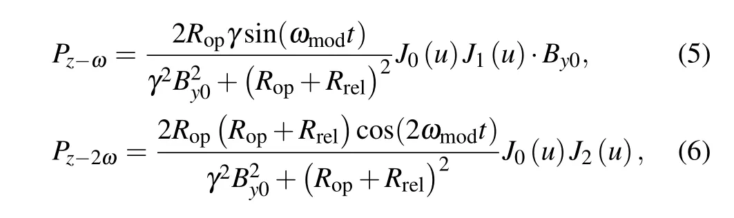
whereJn(n=0,1,2)is then-order Bessel function of the first kind, andu=γBmod/qωmodis the modulation index. Consequently,by combining Eqs.(4)–(6),we can get the demodulation voltage signals at the first and second harmonic
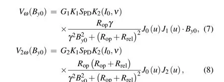
whereG1andG2are the output voltage gain factors for different channels of the lock-in amplifier,K1is the current–voltage conversion coefficient of transimpedance amplifier,SPDis the photosensitivity of photodiodes,andK2is a conversion coefficient between transmitted light intensity and spin polarizationPz

The conventional first harmonic response signal is affected by the incident optical intensityI0,frequencyνand the modulation indexuas indicated in Eq.(7). Based on Eqs.(7)and(8),we introduce the modification method with the correction of the second harmonic response and the corresponding response signal is

As indicated in Eq. (10), response signalVMODshows the improved dynamic range and lower linearity error toBy0for eliminating the nonlinear termγ2B2y0inVω. Meanwhile,in contrast to the first harmonic signalVω, termsK1,SPD,K2(I0,ν)are removed inVMOD,which gives a more stable response signal by suppressing the influence of optical intensityI0and frequencyνfluctuations. In summary, the proposed modification method promises an accurate and stable response signal in a larger measurement range of magnetic fields.
3. Experimental setup and procedures
A potassium spherical glass vapor cell with a diameter of 10 mm was filled with 1.8 amg4He and 0.1 amg N2. The N2acted as the quenching gas to prevent the radiation trapping while the4He efficiently decreased the effect of wall collisions. The vapor cell was electrically heated to 170°C by a printed double-layer resistance wire, generating an atomic number density of 4.97×1013cm-3according to Ref. [31].The heating resistance wire was specially designed to make the current flow in opposite directions between adjacent wires to eliminate the heating-current-induced magnetic field. The vapor cell temperature was stabilized by a proportional-integralderivative (PID) controller at an accuracy of±0.02°C, and the accuracy was obtained by a non-magnetic Pt-1000 temperature sensor that closed to the vapor cell.
The experiments were carried out on a single-beam atomic magnetometer,as shown in Fig.1. The optical pumping beam was generated from an external-cavity diode laser(ECDL, New Focus TLB-6813), and carried into the magnetometer through a single-mode polarization-maintaining fiber.The optical frequency was tuned and locked to the D1 line of potassium at 770.1033 nm (389.2886 THz) by the feedback of a wavelength meter(HighFinesse WS-7). An acousto-optic modulator(AOM,G&H 3080-125)was placed in front of the optical fiber to modulate the light and generate artificial intensity fluctuations. The light emitted from the fiber was expanded and collimated to a diameter of 4 mm, then passed through the polarizer and quarter-wave plate in sequence. The incident intensityI0=6.35 mW/cm2traversed through the vapor cell alongz-direction and was finally exposed to the photodiode.The photosensitivitySPDof the photodiode was about 0.55 A/W at 389.2886 THz.
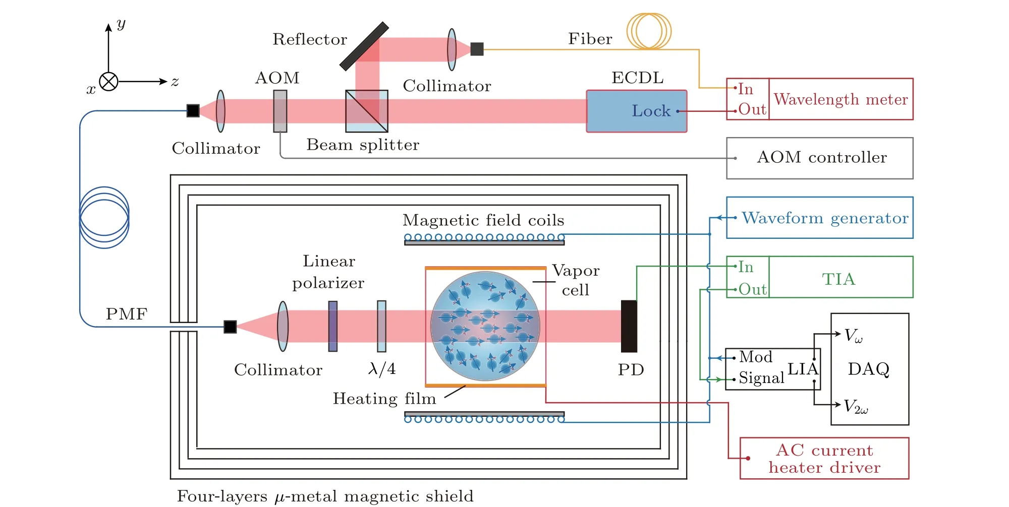
Fig. 1. Schematic of the experimental apparatus. ECDL: external-cavity diode laser, TIA: transimpedance amplifier, LIA: lock-in amplifier, PD:silicon photodiode,DAQ:data acquisition system,λ/4: quarter-wave plate,AOM:acousto-optic modulator,PMF:polarization-maintaining fiber.
The atomic magnetometer was placed inside a four-layers μ-metal magnetic shield, and the internal residual magnetic field was below 2 nT.Before running the experiment,the magnetic field surrounding the vapor cell was compensated to near zero-field (typically below 1 pT) by triaxial magnetic field coils integrated inside the magnetometer driven by the waveform generators (Keysight 33522B). The response signalVω,V2ωto magnetic fieldBy0was extracted using the digital lockin amplifier (Zurich Instruments MFLI) following the process: the lock-in amplifier generated the modulation voltage signalVmodsin(ωmodt) and applied to they-axis coil through a series resistance to produce the modulation magnetic fieldBmodsin(ωmodt) whereBmod=110 nT,ωmod=900 Hz; the spin polarization evolved in the modulation magnetic field,yielding the variation of transmitted light intensityIas indicated in Eq. (4); the corresponding light intensity variations were detected by a silicon photodiode and converted to the voltage signal by the transimpedance amplifier (Thorlabs PDA200C) with conversion coefficientK1subsequently; this voltage signal was finally sent to the lock-in amplifier for demodulation at first and second harmonic, generating the corresponding voltage responseVωandV2ωwith gain factorG1andG2, respectively. In practice, we madeG1=G2in the subsequent experiments.
The queen then began to put the room in order and prepare food, so that when the man came home he found everything neat and tidy, and this seemed to give him some pleasure
To investigate the magnetometer’s dynamic range and linearity, a sweep magnetic field ranging in±30 nT was applied to they-axis coil. The corresponding response voltagesVωandV2ωwere recorded simultaneously withBy0by the data acquisition system (NI PXIe-4464) at the sampling rate of 1 kHz. Furthermore, to estimate the stability of magnetometer’s response signal under optical intensity and frequency fluctuations,the artificial variations were applied to the incident light. For optical intensity fluctuations, a 40 mVpp triangular modulation at 1 Hz was applied to the AOM,generating a 5%variation of optical intensity,resulting inI0varying from 6.2 mW/cm2to 6.51 mW/cm2periodically. For optical frequency fluctuations, by controlling the piezoelectric transducer(PZT)voltage inside the ECDL,the incident optical frequency was varied atν389.2886 THz±15 GHz.Additionally,a 100 pT sinusoidal calibration magnetic field at 31 Hz was applied along they-axis, and the corresponding peak-to-peak amplitude in the response signal was extracted to evaluate the signal stability under optical intensity and frequency fluctuations.
4. Results and discussion
4.1. Dynamic range and linearity
As shown in Fig.2,the first and second harmonic signalsVωandV2ωextracted from the lock-in amplifier were illustrated with black and blue lines. The modification response in Fig. 2 with the red line referred to the response signal calculated through our modification method as indicated in Eq.(10).By adjusting the voltage gain factorG1andG2,the modification response was made consistently with the first harmonic response to the same magnetic fieldBy0.

Fig.2. The first harmonic(black line)and second harmonic(blue line)responses of the magnetic field By0 and the modification response(red line)calculated from Eq.(10). The shaded areas of the curves indicated multiple measurement errors.
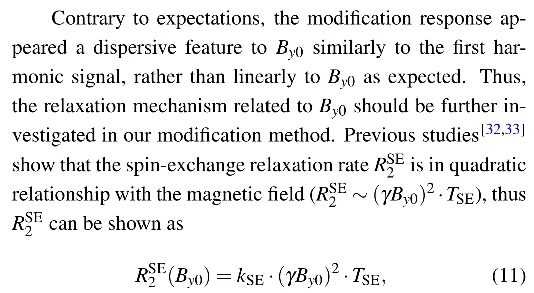

Referring to the study by Reaet al.,[26]the dynamic range of the atomic magnetometer was defined as the measurement range where the linearity error was less than 5%. As shown in Fig.3(a)with the shaded region,the calibrated first harmonic response showed the dynamic range of 2 nT,while the modification response remained a linear response over the range of 10 nT.
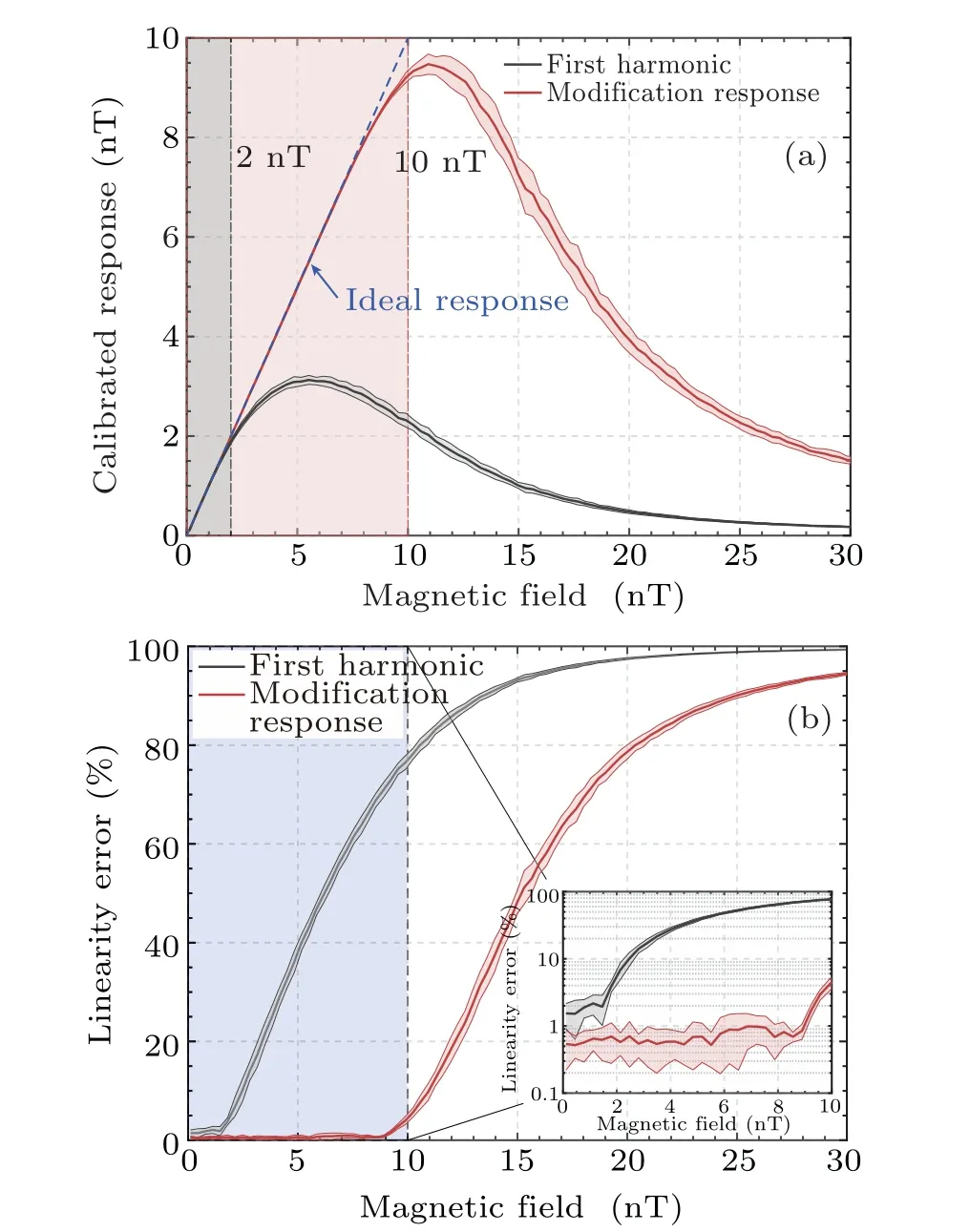
Fig. 3. (a) Calibrated response of conventional first harmonic (black line) and modification response (red line); (b) linearity error of both conventional model(black line)and modification model(red line); inset: linearity error within 10 nT range with y-axis in logarithmic scale.
Figure 3(b)demonstrated the linearity errorδLcomparison of the first harmonicVωand modification responseVMOD.It was apparent that the linearity error of the first harmonic response increased rapidly when the magnetic field exceeded its dynamic range of 2 nT, while the modification response maintained its linearity within 10 nT. Notably, the modification response showed a relatively small linearity error within the dynamic range of 10 nT,givingδL<1%as shown in the inset.
4.2. Response signal stability
The proposed modification responseVMODshowed the suppression of response instability induced by optical intensityI0and frequencyνfluctuations as indicated in Eq. (12).Firstly, the response signal stability was investigated by applying artificial fluctuations on optical intensity.As indicated in Fig. 4, the first harmonic and modification responses were recorded with black and red lines,against the variation of 5%in optical intensity with the blue line. It was seen from the figure that the instability of the first harmonic influenced by optical intensity fluctuations was suppressed in our modification method, which gave a stable response signal as shown with the red line.
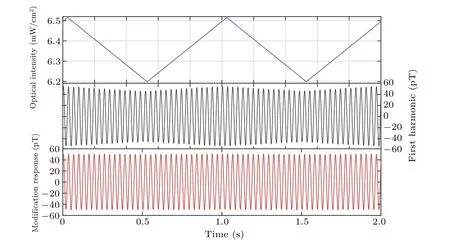
Fig.4. First harmonic(black line)and the modification response curves(red line)to 100 pT sinusoidal magnetic field at 31 Hz under the 5%optical intensity fluctuations(blue line).

Fig.5.Linearity error of the first harmonic response(red line)and modification response(black line)induced by optical intensity fluctuations calculated by Eq.(13).
Moreover, the linearity error was taken to quantify the suppression of optical intensity fluctuations. The peak-topeak amplitude of the response signal in a period was taken asSresponsefor both first harmonicVωand modification responseVMODandSsignalwas the averaged peak-to-peak amplitude ofVωandVMODduring the measurement time, respectively. As shown in Fig. 5, the first harmonic response suffered a 15%variation and showed a trend consistent with optical intensity fluctuations. As a comparison, the linearity error of modification response was maintained lower than 1%, independent from the influence of optical intensity fluctuations.
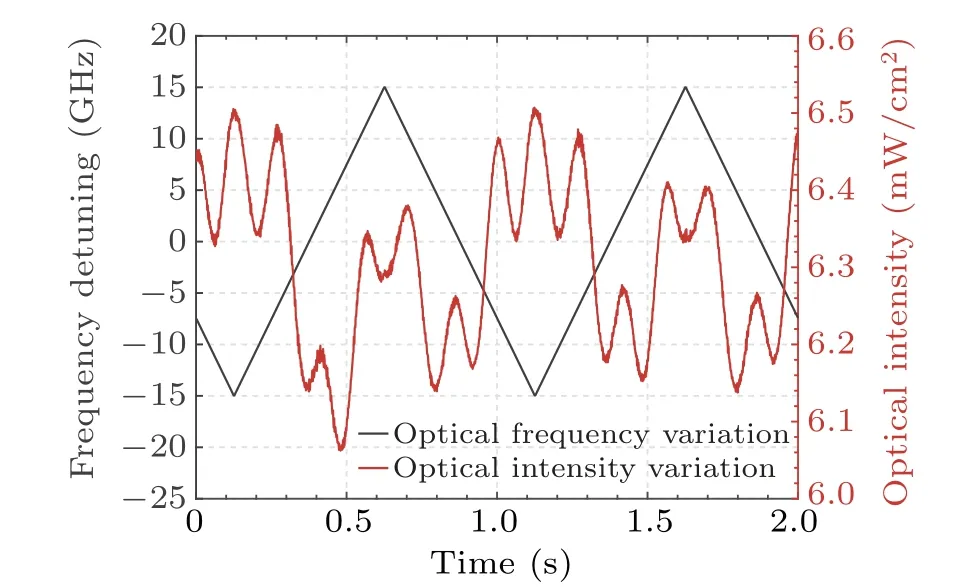
Fig. 6. Modulation on the incident optical frequency with 1 Hz triangular wave(black line)and the accompanied optical intensity noise(red line).
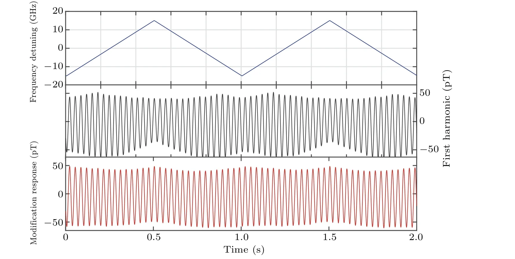
Fig.7. First harmonic response(black line)and the modification response(red line)to the 100 pT sinusoidal magnetic field at 31 Hz under the influence of the optical frequency fluctuations at±15 GHz(blue line).
Moreover,the influence of optical frequency fluctuations on the response signal was studied. By controlling the PZT voltage inside the ECDL,a linear optical frequency variation of 389.2886 THz±15 GHz was obtained, accompanied by undesired optical intensity noise,as shown in Fig.6. The unexpected optical intensity fluctuations were caused by the limitation of the ECDL,but they would not have fatal impacts on subsequent analysis.
As shown in Fig. 7, with the combined influence of optical frequency and intensity fluctuations, the first harmonic responseVωchanged significantly while the modification responseVMODshowed slight variations. The linearity errorδLof the first harmonic response varied 38% under the optical frequency fluctuations,as demonstrated in Fig.8. On the contrary,the modification response maintained a level of 8%under the combined effects of optical intensity and frequency variations. In addition, the asymmetry of the linearity error between±15 GHz frequency detuning in Fig.8 was because the magnetometer worked with the slight frequency detuning(about 7 GHz redshift in our experiment)for the optimal performance.

Fig.8. First harmonic(red line)and modification(black line)linearity error caused by optical frequency variation.
Finally,the noise spectral density averaged for 2 minutes of both the first harmonicVω(in red line) and the modification responseVMOD(in red dashed line)was shown in Fig.9.As seen, the noise spectral density of the proposed modification response was 8 fT/Hz1/2, which may be limited by the magnetic noise of the magnetic shield,[35]consistently with the first harmonic response signal.
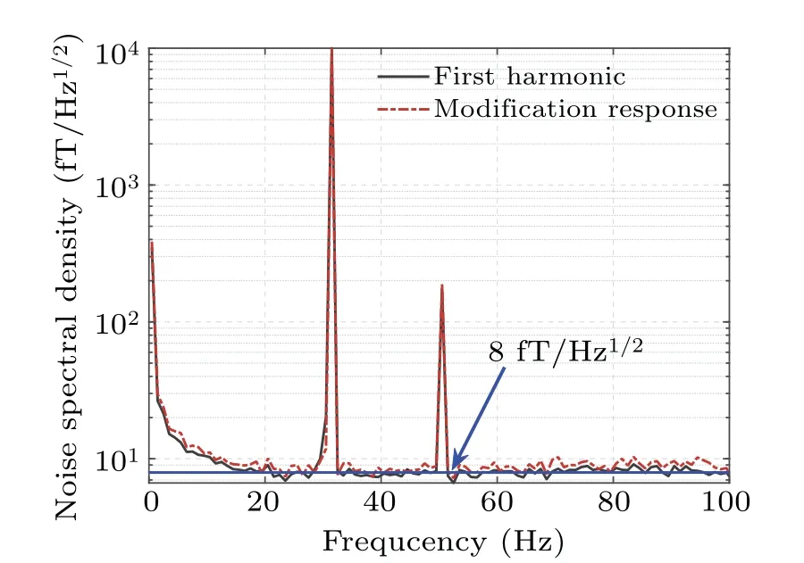
Fig.9.Noise spectral densities of the conventional response and our modification method.The peak at 31 Hz was the calibration signal we applied,the peak at 50 Hz Hz was the power frequency of the environment, and the blue line was a fit to the atomic magnetometer noise floor.
5. Conclusion
In this study, we develop a comprehensive response model for magnetic field measurement in zero-field singlebeam atomic magnetometer. Then the modification method for magnetometer’s response that introduces the second harmonic correction is proposed, which is advantageous in dynamic range expansion,linearity error reduction,and response signal stability. The experiments showed that the dynamic range was expanded to 10 nT, 5-fold larger than 2 nT in the conventional method. Furthermore, the linearity error of the proposed method was maintained at 1%in the dynamic range,five times lower than the first harmonic response. In addition,when optical intensity fluctuated at 5%and frequency detuned between±15 GHz, the response signal was maintained at intensity-related bias less than 1%and frequency-related bias less than 8%, whereas the conventional method suffers instability of 15%and 38%,respectively.
Additionally,the modified response is as sensitive as the first harmonic signal, ensuring high-sensitive and accurate magnetic field measurement. Furthermore, our modification method operated in real-time without introducing extra interferences to the environment,which is advantageous for the applications of MEG and MCG,where sensor arrays are utilized.
Acknowledgements
The authors would like to give special thanks to Feifan Tan for her encouragement.
Project supported by the National Key R&D Program of China(Grant No.2018YFB2002405)and the National Natural Science Foundation of China(Grant No.61903013).
猜你喜欢
东坡赤壁诗词(2022年4期)2022-10-30
故事会(2022年11期)2022-06-02
电脑知识与技术(2022年11期)2022-05-31
人才资源开发(2022年9期)2022-05-28
电脑知识与技术(2022年9期)2022-05-10
Plasma Science and Technology(2022年2期)2022-03-10
分忧(2021年7期)2021-07-22
Plasma Science and Technology(2021年4期)2021-04-22
寻根(2020年1期)2020-04-07
辽金历史与考古(2019年0期)2020-01-06

- Chinese Physics B的其它文章
- A design of resonant cavity with an improved coupling-adjusting mechanism for the W-band EPR spectrometer
- Photoreflectance system based on vacuum ultraviolet laser at 177.3 nm
- Topological photonic states in gyromagnetic photonic crystals:Physics,properties,and applications
- Structure of continuous matrix product operator for transverse field Ising model: An analytic and numerical study
- Riemann–Hilbert approach and N double-pole solutions for a nonlinear Schr¨odinger-type equation
- Diffusion dynamics in branched spherical structure