Tensor Train Random Projection

Yani Feng,Kejun Tang,Lianxing He,Pingqiang Zhou and Qifeng Liao,★

1School of Information Science and Technology,ShanghaiTech University,Shanghai,201210,China

2Peng Cheng Laboratory,Shenzhen,518055,China

3Innovation Academy for Microsatellites of Chinese Academy of Sciences,Shanghai,201210,China

ABSTRACT This work proposes a Tensor Train Random Projection(TTRP)method for dimension reduction,where pairwise distances can be approximately preserved.Our TTRP is systematically constructed through a Tensor Train(TT)representation with TT-ranks equal to one.Based on the tensor train format,this random projection method can speed up the dimension reduction procedure for high-dimensional datasets and requires fewer storage costs with little loss in accuracy,compared with existing methods.We provide a theoretical analysis of the bias and the variance of TTRP,which shows that this approach is an expected isometric projection with bounded variance,and we show that the scaling Rademacher variable is an optimal choice for generating the corresponding TT-cores.Detailed numerical experiments with synthetic datasets and the MNIST dataset are conducted to demonstrate the efficiency of TTRP.

KEYWORDS Tensor Train;random projection;dimension reduction

1 Introduction

Dimension reduction is a fundamental concept in science and engineering for feature extraction and data visualization.Exploring the low-dimensional structures of high-dimensional data attracts broad attention.Popular dimension reduction methods include Principal Component Analysis(PCA)[1,2],Non-negative Matrix Factorization(NMF)[3],and t-distributed Stochastic Neighbor Embedding(t-SNE)[4].A main procedure in dimension reduction is to build a linear or nonlinear mapping from a high-dimensional space to a low-dimensional one,which keeps important properties of the high-dimensional space,such as the distance between any two points[5].

The Random Projection(RP)is a widely used method for dimension reduction.It is well-known that the Johnson-Lindenstrauss(JL)transformation[6,7]can nearly preserve the distance between two points after a random projectionf,which is typically called isometry property.The isometry property can be used to achieve the nearest neighbor search in high-dimensional datasets[8,9].It can also be used to build the Restricted Isometry Property (RIP) in compressed sensing [10,11],where a sparse signal can be reconstructed under a linear random projection[12].The JL lemma[6]tells us that there exists a nearly isometry mappingf,which maps high-dimensional datasets into a lower dimensional space.Typically,a choice for the mappingfis the linear random projection.

wherex∈RN,andR∈RM×Nis a matrix whose entries are drawn from the mean zero and variance one Gaussian distribution,denoted byN (0,1).We call it Gaussian random projection (Gaussian RP).The storage of matrixRin Eq.(1) isO(MN)and the cost of computingRxin Eq.(1) isO(MN).However,with largeMandN,this construction is computationally infeasible.To alleviate the difficulty,the sparse random projection method[13]and the very sparse random projection method[14]are proposed,where the random projection is constructed by a sparse random matrix.Thus the storage and the computational cost can be reduced.

To be specific,Achlioptas [13] replaced the dense matrixRby a sparse matrix whose entries follows:

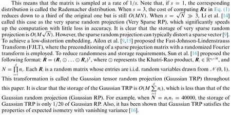
Recently,using matrix or tensor decomposition to reduce the storage of projection matrices is proposed in [17,18].The main idea of these methods is to split the projection matrix into some small scale matrices or tensors.In this work,we focus on the low rank tensor train representation to construct the random projectionf.Tensor decompositions are widely used for data compression[5,19–24].The Tensor Train (TT) decomposition,also called Matrix Product States (MPS) [25–28],gives the following benefits—low rank TT-formats can provide compact representations of projection matrices and efficient basic linear algebra operations of matrix-by-vector products[29].Based on these benefits,we propose a Tensor Train Random Projection(TTRP)method,which requires significantly smaller storage and computational costs compared with existing methods (e.g.,Gaussian TRP [16],Very Sparse RP [14] and Gaussian RP [30]).We note that constructing projection matrices using Tensor Train(TT)and Canonical Polyadic(CP)decompositions based on Gaussian random variables is proposed in[31].The main contributions of our work are three-fold:first our TTRP is conducted based on a rank-one TT-format,which significantly reduces the storage of projection matrices;second,we provide a novel construction procedure for the rank-one TT-format in our TTRP based on i.i.d.Rademacher random variables; third,we prove that our construction of TTRP is unbiased with bounded variance.

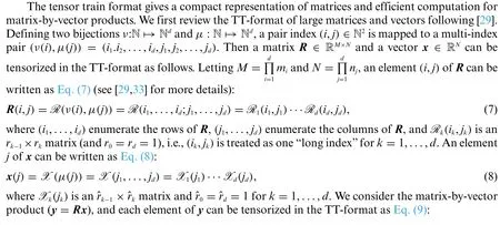
The rest of the paper is organized as follows.The tensor train format is introduced in Section 2.Details of our TTRP approach are introduced in Section 3,where we prove that the approach is an expected isometric projection with bounded variance.In Section 4,we demonstrate the efficiency of TTRP with datasets including synthetic,MNIST.Finally Section 5 concludes the paper.

2 Tensor Train Format

The Kronecker product conforms the following laws[32]:

2.1 Tensor Train Decomposition

Tensor Train(TT)decomposition[29]is a generalization of Singular Value Decomposition(SVD)from matrices to tensors.TT decomposition provides a compact representation for tensors,and allows for efficient application of linear algebra operations(discussed in Section 2.2 and Section 2.3).

Given ad-th order tensorG∈Rn1×··×ndand a vectorg(vector format ofG) ,the tensor train decomposition[29]is

whereν:NNdis a bijection,Gk∈Rrk-1×nk×rkare called TT-cores,Gk(ik)∈Rrk-1×rkis a slice ofGk,fork= 1,2,...,d,ik= 1,...,nk,and the“boundary condition”isr0=rd= 1.The tensorGis said to be in the TT-format if each element ofGcan be represented by Eq.(6).The vector[r0,r1,r2,...,rd]is referred to as TT-ranks.LetGk(αk-1,ik,αk)represent the element ofGk(ik)in the position(αk-1,αk).In the index form,the decomposition(6)is rewritten as the following TT-format:

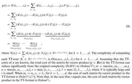
To look more closely to Eq.(6),an elementG(i1,i2,...,id)is represented by a sequence of matrixby-vector products.Fig.1 illustrates the tensor train decomposition.It can be seen that the key ingredient in tensor train (TT) decomposition is the TT-ranks.The TT-format only usesO(ndr2)memory toO(nd)elements,wheren= max {n1,...,nd} andr= max {r0,r1,...,rd}.Although the storage reduction is efficient only if the TT-rank is small,tensors in data science and machine learning typically have low TT-ranks.Moreover,one can apply the TT-format to basic linear algebra operations,such as matrix-by-vector products,scalar multiplications,etc.In later section,it is shown that this can reduce the computational cost significantly when the data have low rank structures(see[29]for details).

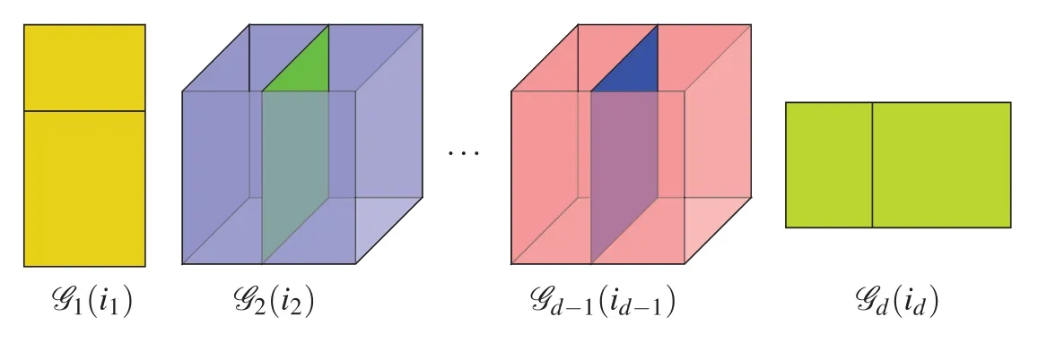
Figure 1:Tensor train format(TT-format):extract an element G(i1,i2,...,id)via a sequence of matrixbyvector product

2.2 Tensorizing Matrix-by-Vector Products

2.3 Basic Operations in the TT-Format

In Section 2.2,the product of matrixRand vectorxwhich are both in the TT-format,is conducted efficiently.In the TT-format,many important operations can be readily implemented.For instance,computing the Euclidean distance between two vectors in the TT-format is more efficient with less storage than directly computing the Euclidean distance in standard matrix and vector formats.In the following Eqs.(10)–(15),some important operations in the TT-format are discussed.

where

where

and we obtain

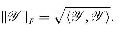
The Frobenius norm of a tensorYis defined by

Computing the distance between tensorYand tensorin the TT-format is computationally efficient by applying the dot product Eqs.(11)and(12),

The complexity of computing the distance is alsoO(dmr3).Algorithm 1 gives more details about computing Eq.(16)based on Frobenius norm‖

Algorithm 1:Distance based on Frobenius norm W:=‖‖Y - ^Y‖‖F =images/BZ_429_1648_839_1686_885.png〈Y - ^Y,Y - ^Y〉Input:TT-cores Yk of tensor Y and TT-cores ^Yk of tensor ^Y,for k=1,...,d.1: Compute Z:=Y - ^Y.▷O(mr)by(10)2: Compute v1:=images/BZ_429_660_1033_708_1079.pngi1 Z1(i1)⊗Z1(i1).▷O(mr2)by Eq.(13)3: for k=2:d-1 do 4: Compute pk(ik)=vk-1(Zk(ik)⊗Zk(ik)).▷O(r3)by Eq.(15)5: Compute vk:=images/BZ_429_730_1230_778_1276.pngik pk(ik).▷O(mr3)by Eq.(14)6: end for 7: Compute pd(id)=vd-1(Zd(id)⊗Zd(id)).▷O(r2)by Eq.(15)8: Compute vd:=images/BZ_429_661_1427_709_1473.pngid pd(id).▷O(mr2)by Eq.(14)Output:Distance W:=images/BZ_429_768_1522_806_1568.png〈Y - ^Y,Y - ^Y〉=■vd.

In summary,just merging the cores of two tensors in the TT-format can perform the subtraction of two tensors instead of directly subtraction of two tensors in standard tensor format.A sequence of matrix-by-vector products can achieve the dot product of two tensors in the TT-format.The cost of computing the distance between two tensors in the TT-format,reduces from the original complexity

3 Tensor Train Random Projection

Due to the computational efficiency of TT-format discussed above,we consider the TT-format to construct projection matrices.Our tensor train random projection is defined as follows.

Definition 3.1.(Tensor Train Random Projection).For a data pointx∈ RN,our tensor train random projection(TTRP)is

Proof.Denotingy=Rxgives

where Eq.(20) is derived using Eqs.(3) and (19),and then combining Eq.(20) and using the independence of TT-coresR1,...,Rdgive Eq.(21).Thek-th term of the right hand side of Eq.(21),fork=1,...,d,can be computed by

Substituting Eq.(27)into Eq.(18),it concludes that

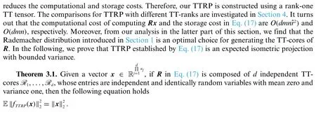
Theorem 3.2.Given a vector,ifRin Eq.(17)is composed ofdindependent TT-coresR1,...,Rd,whose entries are independent and identically random variables with mean zero,variance one,with the same fourth momentΔandM:= maxi=1,...,N|x(i)|,m= max{m1,m2,...,md},n=max{n1,n2,...,nd},then

Proof.By the property of the variance and using Theorem 3.1,

where note that E[y2(i)y2(j)]E[y2(i)]E[y2(j)] in general and a simple example can be found in Appendix A.

We compute the first term of the right hand side of Eq.(29),

wherey(i)=Y(i1,...,id),applying Eq.(3)to Eq.(30)obtains Eq.(31),and we derive Eq.(32)from Eq.(31)by the independence of TT-cores

Considering thek-th term of the right hand side of Eq.(32),fork=1,...,d,we obtain that

where we infer Eq.(34)from Eq.(33)by scalar property ofRk(ik,jk),Eq.(35)is obtained by Eq.(4)and the independence of TT-cores,and denoting the fourth momentΔ: =we deduce Eq.(36)by the assumption=1,fork=1,...,d.

Substituting Eq.(36)into Eq.(32),it implies that

where denotingM: = maxi=1,...,N|x(i)|,n= max{n1,n2,...,nd},we derive Eq.(38) from Eq.(37) by Eq.(3).

Similarly,the second term E[y2(i)y2(j)] of the right hand side of Eq.(29),fori≠j,ν(i)=(i1,i2,...,id)≠ν(j)=,is obtained by

Ifik≠,fork=1,...,d,then thek-th term of the right hand side of Eq.(40)is computed by E[Yk(ik)⊗Yk(ik)⊗Yk()⊗Yk()]

Similarly,if fork∈S⊆{1,...,d},|S|=l,ik≠,and fork∈,ik=,then

Hence,combining Eqs.(42)and(43)gives

wherem=max{m1,m2,...,md}.

Therefore,using Eqs.(39)and(44)deduces

In summary,substituting Eq.(45)into Eq.(28)implies

One can see that the bound of the variance Eq.(46)is reduced asMincreases,which is expected.WhenM=mdandN=nd,we have

Note that asmincreases,the upper bound in Eq.(47)tends to≥0,and this upper bound vanishes asMincreases if and only ifx(1)=x(2)=...=x(N).Also,the upper bound in Eq.(46)is affected by the fourth momentΔ==To keep the expected isometry,we need=1.Note that when the TT-cores follow the Rademacher distribution,i.e.,=0,the fourth momentΔin Eq.(46)achieves the minimum.So,the Rademacher distribution is an optimal choice for generating the TT-cores,and we set the Rademacher distribution to be our default choice for constructing TTRP(Definition 3.1).

Proposition 3.1.(Hypercontractivity[35])Consider a degreeqpolynomialf(Y)=f (Y1,...,Yn)of independent centered Gaussian or Rademacher random variablesY1,...,Yn.Then for anyλ ＞0

where Var([f(Y)])is the variance of the random variablef(Y)andK ＞0 is an absolute constant.

Proposition 3.1 extends the Hanson-Wright inequality whose proof can be found in[35].

Proposition 3.2.LetfTTRP:RNRMbe the tensor train random projection defined by Eq.(17).Suppose that fori= 1,...,d,all entries of TT-coresRiare independent standard Gaussian or Rademacher random variables,with the same fourth momentΔandM: = maxi=1,...,N|x(i)|,m=max{m1,m2,...,md},n= max{n1,n2,...,nd}.For anyx∈ RN,there exist absolute constantsCandK ＞0 such that the following claim holds

Proof.According to Theorem 3.1,Sinceis a polynomial of degree 2dof independent standard Gaussian or Radamecher random variables,which are the entries of TTcoresRi,fori=1,...,d,we apply Proposition 3.1 and Theorem 3.2 to obtain

whereM=maxi=1,...,N|x(i)|and then

We note that the upper bound in Proposition 3.2 is not tight,as it involves the dimensionality of datasets(N).To give a tight bound independent of the dimensionality of datasets for the corresponding concentration inequality is our future work.

The procedure of TTRP is summarized in Algorithm 2.For the input of this algorithm,the TTranks ofR(the tensorized version of the projection matrixRin Eq.(17))are set to one,and from our above analysis,we generate entries of the corresponding TT-coresthrough the Rademacher distribution.For a given data pointxin the TT-format,Algorithm 2 gives the TT-cores of the corresponding output,and each element offTTRP(x)in Eq.(17)can be represented as

whereνis a bijection from N to Nd.

4 Numerical Experiments

We demonstrate the efficiency of TTRP using synthetic datasets and the MNIST dataset[36].The quality of isometry is a key factor to assess the performance of random projection methods,which in our numerical studies is estimated by the ratio of the pairwise distance:

wheren0is the number of data points.Since the output of our TTRP procedure (see Algorithm 2)is in the TT-format,it is efficient to apply TT-format operations to compute the pairwise distance of Eq.(48)through Algorithm 1.In order to obtain the average performance of isometry,we repeat numerical experiments 100 times(different realizations for TT-cores)and estimate the mean and the variance for the ratio of the pairwise distance using these samples.The rest of this section is organized as follows.First,through a synthetic dataset,the effect of different TT-ranks of the tensorized versionRofRin Eq.(17)is shown,which leads to our motivation of setting the TT-ranks to be one.After that,we focus on the situation with TT-ranks equal to one,and test the effect of different distributions of TT-cores.Finally,based on both high-dimensional synthetic and MNIST datasets,our TTRP are compared with related projection methods,including Gaussian TRP [16],Very Sparse RP [14] and Gaussian RP[30].All results reported below are obtained in MATLAB with TT-Toolbox 2.2.2(https://github.com/oseledets/TT-Toolbox).

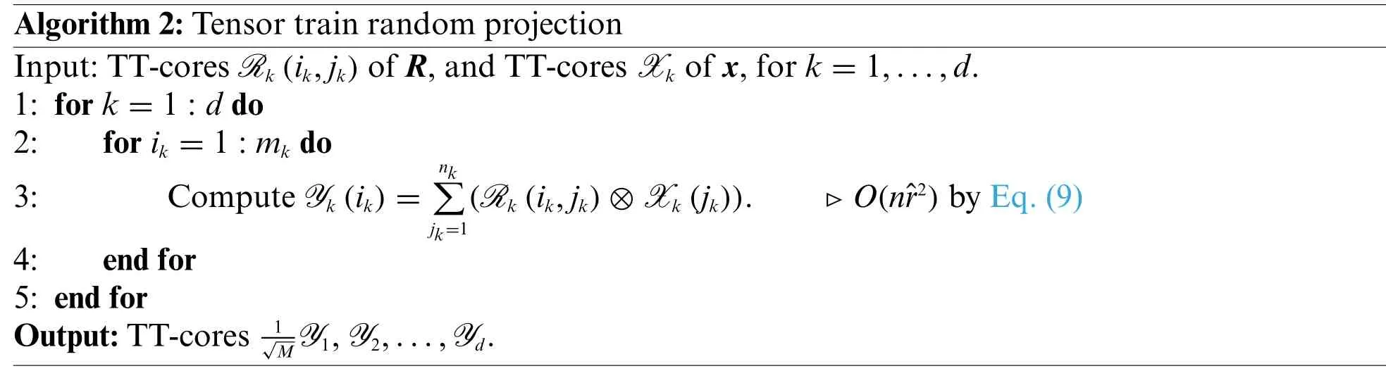
Algorithm 2:Tensor train random projection Input:TT-cores Rk(ik,jk)of R,and TT-cores Xk of x,for k=1,...,d.1: for k=1:d do 2: for ik =1:mk do 3: Compute Yk(ik)=nkimages/BZ_437_894_1335_942_1381.pngjk=1(Rk(ik,jk)⊗Xk(jk)).▷O(nˆr2)by Eq.(9)4: end for 5: end for Output:TT-cores 1■MY1,Y2,...,Yd.

4.1 Effect of Different TT-Ranks

In Definition 3.1,we set the TT-ranks to be one.To explain our motivation of this settting,we investigate the effect of different TT-ranks—we herein consider the situation that the TT-ranks taker0=rd= 1,rk=r,k= 1,...,d-1,where the rankr∈{1,2,...},and we keep other settings in Definition 3.1 unchanged.For comparison,two different distributions are considered to generate the TT-cores in this part—the Rademacher distribution (our default optimal choice) and the Gaussian distribution,and the corresponding tensor train projection is denoted by rank-rTTRP and Gaussian TT,respectively.To keep the expected isometry of rank-rTTRP,the entries of TT-coresR1andRdare drawn from 1/r1/4or -1/r1/4with equal probability,and each element ofRk,k= 2,..,d-1 is uniformly and independently drawn from 1/r1/2or-1/r1/2.For Gaussian TT,Rkfork=2,...,d-1 andk=1,dare drawn fromNandN,respectively.

Two synthetic datasets with dimensionN=1000 are generated(the size of the first one isn0=10 and that of the second one isn0= 50),where each entry of vectors (each vector is a sample in the synthetic dataset)is independently generated throughN (0,1).In this test problem,we set the reduced dimension to beM= 24,and the dimensions of the corresponding tensor representations are set tom1= 4,m2= 3,m3= 2 andn1=n2=n3= 10 (M=m1m2m3andN=n1n2n3).Fig.2 shows the ratio of the pairwise distance of the two projection methods(computed through Eq.(48)).It can be seen that the estimated mean of ratio of the pairwise distance of rank-rTTRP is typically more close to one than that of Gaussian TT,i.e.,rank-rTTRP has advantages for keeping the pairwise distances.Clearly,for a given rank in Fig.2,the estimated variance of the pairwise distance of rank-rTTRP is smaller than that of Gaussian TT.Moreover,focusing on rank-rTTRP,the results of both the mean and the variance are not significantly different for different TT-ranks.In order to reduce the storage,we only focus on the rank-one case(as in Definition 3.1)in the rest of this paper.

Figure 2:Effect of different ranks based on synthetic data(M =24,N =1000,m1 =4,m2 =3,m3 =2,n1 =n2 =n3 =10)

4.2 Effect of Different TT-Cores

Two synthetic datasets are tested to assess the effect of different distributions for TT-cores,whose sizes aren0= 10 andn0= 50,respectively,with dimensionN= 2500,whose elements are sampled from the standard Gaussian distribution.The following three distributions are investigated to construct TTRP(see Definition 3.1),which include the Rademacher distribution(our default choice),the standard Gaussian distribution,and the 1/3-sparse distribution(i.e.,s= 3 in Eq.(2)),while the corresponding projection methods are denoted by TTRP-RD,TTRP-N (0,1),and TTRP-1/3-sparse,respectively.For this test problem,three TT-cores are utilized form1=M/2,m2= 2,m3= 1 andn1= 25,n2= 10,n3= 10.Fig.3 shows that the estimated mean of the ratio of the pairwise distance for TTRP-RD is very close to one,and the estimated variance of TTRP-RD is at least one order of magnitude smaller than that of TTRP-N (0,1)and TTRP-1/3-sparse.These results are consist with Theorem 3.2.In the rest of this paper,we focus on our default choice for TTRP—the TT-ranks are set to one,and each element of TT-cores is independently sampled through the Rademacher distribution.

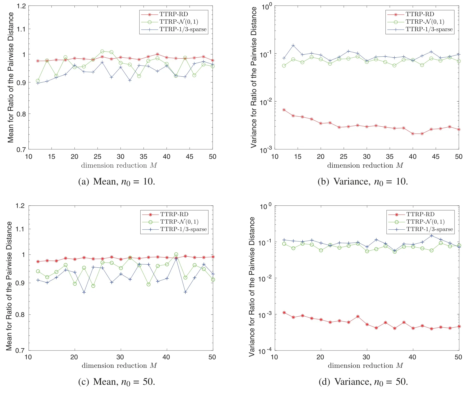
Figure 3:Three test distributions for TT-cores based on synthetic data(N=2500)

4.3 Comparison with Gaussian TRP,Very Sparse RP and Gaussian RP

The storage of the projection matrix and the cost of computingRx(see Eq.(17))of our TTRP(TTranks equal one),Gaussian TRP[16],Very Sparse RP[14]and Gaussian RP[30],are shown in Table 1,whereR∈RM×N,M=,m= max{m1,m2,...,md}andn= max{n1,n2,...,nd}.Note that the matrixRin Eq.(17)is tensorized in the TT-format,and TTRP is efficiently achieved by the matrix-by-vector products in the TT-format(see Eq.(9)).From Table 1,it is clear that our TTRP has the smallest storage cost and requires the smallest computational cost for computingRx.

Table 1: The comparison of the storage and the computational costs

Two synthetic datasets with sizen0= 10 are tested—the dimension of the first one isN= 2500 and that of the second one isN= 104;each entry of the samples is independently generated throughN (0,1).For TTRP and Gaussian TRP,the dimensions of tensor representations are set to: forN= 2500,we setn1= 25,n2= 10,n3= 10,m1=M/2,m2= 2,m3= 1; forN= 104,we setn1=n2= 25,n3=n4= 4,m1=M/2,m2= 2,m3= 1,m4= 1,whereMis the reduced dimension.We again focus on the ratio of the pairwise distance (putting the outputs of different projection methods into Eq.(48)),and estimate the mean and the variance for the ratio of the pairwise distance through repeating numerical experiments 100 times(different realizations for constructing the random projections,e.g.,different realizations of the Rademacher distribution for TTRP).

Fig.4 shows that the performance of TTRP is very close to that of sparse RP and Gaussian RP,while the variance for Gaussian TRP is larger than that for the other three projection methods.Moreover,the variance for TTRP basically reduces as the dimensionMincreases,which is consistent with Theorem 3.2.To be further,more details are given for the case withM= 24 andN= 104in Tables 2 and 3,where the value of storage is the number of nonzero entries that need to be stored.It turns out that TTRP with fewer storage costs achieves a competitive performance compared with Very Sparse RP and Gaussian RP.In addition,from Table 3,ford ＞2,the variance of TTRP is clearly smaller than that of Gaussian TRP,and the storage cost of TTRP is much smaller than that of Gaussian TRP.

Figure 4:Mean and variance for the ratio of the pairwise distance,synthetic data

Table 2:The comparison of mean and variance for the ratio of the pairwise distance,and storage,for Gaussian RP and Very Sparse RP(M =24 and N =104)

Table 3:The comparison of mean and variance for the ratio of the pairwise distance,and storage,for Gaussian TRP and TTRP(M =24 and N =104)

Next the CPU times for projecting a data point using the four methods(TTRP,Gaussian TRP,Very Sparse RP and Gaussian RP)are assessed.Here,we set the reduced dimensionM= 1000,and test four cases withN=104,N=105,N=2×105andN=106,respectively.The dimensions of the tensorized output is set tom1=m2=m3= 10(such thatM=m1m2m3),and the dimensions of the corresponding tensor representations of the original data points are set to:forN=104,n1=25,n2=25,n3= 16;forN= 105,n1= 50,n2= 50,n3= 40;forN= 2×105,n1= 80,n2= 50,n3= 50;forN= 106,n1=n2=n3= 100.For each case,given a data point of which elements are sampled from the standard Gaussian distribution,the simulation of projecting it to the reduced dimensional space is repeated 100 times(different realizations for constructing the random projections),and the CPU time is defined to be the average time of these 100 simulations.Fig.5 shows the CPU times,where the results are obtained in MATLAB on a workstation with Intel(R) Xeon(R) Gold 6130 CPU.It is clear that the computational cost of our TTRP is much smaller than those of Gaussian TRP and Gaussian RP for different data dimensionN.Note that as the data dimensionNincreases,the computational costs of Gaussian TRP and Gaussian RP grow rapidly,while the computational cost of our TTRP grows slowly.When the data dimension is large(e.g.,N= 106in Fig.5),the CPU time of TTRP becomes smaller than that of Very Sparse RP,which is consistent with the results in Table 1.

Figure 5:A comparison of CPU time for different random projections(M=1000)

Finally,we validate the performance of our TTRP approach using the MNIST dataset [36].From MNIST,we randomly taken0= 50 data points,each of which is a vector with dimensionN= 784.We consider two cases for the dimensions of tensor representations: in the first case,we setm1=M/2,m2= 2,n1= 196,n2= 4,and in the second case,we setm1=M/2,m2= 2,m3= 1,n1= 49,n2= 4,n3= 4.Fig.6 shows the properties of isometry and bounded variance of different random projections on MNIST.It can be seen that TTRP satisfies the isometry property with bounded variance.Although Gaussian RP has the smallest variance (note that it is not based on the tensor format),its computational and storage costs are large(see Fig.5).It is clear that as the reduced dimensionMincreases,the variances of the four methods reduce,and the variance of our TTRP is close to that of Very Sparse RP.

Figure 6:Isometry and variance quality for MNIST data(N=784)

5 Conclusion

Random projection plays a fundamental role in conducting dimension reduction for highdimensional datasets,where pairwise distances need to be approximately preserved.With a focus on efficient tensorized computation,this paper develops a tensor train random projection (TTRP)method.Based on our analysis for the bias and the variance,TTRP is proven to be an expected isometric projection with bounded variance.From the analysis in Theorem 3.2,the Rademacher distribution is shown to be an optimal choice to generate the TT-cores of TTRP.For computational convenience,the TT-ranks of TTRP are set to one,while from our numerical results,we show that different TT-ranks do not lead to significant results for the mean and the variance of the ratio of the pairwise distance.Our detailed numerical studies show that,compared with standard projection methods,our TTRP with the default setting(TT-ranks equal one and TT-cores are generated through the Rademacher distribution),requires significantly smaller storage and computational costs to achieve a competitive performance.From numerical results,we also find that our TTRP has smaller variances than tensor train random projection methods based on Gaussian distributions.Even though we have proven the properties of the mean and the variance of TTRP and the numerical results show that TTRP is efficient,the upper bound in Proposition 3.2 involves the dimensionality of datasets(N),and our future work is to give a tight bound independent of the dimensionality of datasets for the concentration inequality.

Appendix A

Example forE[y2(i)y2(j)]≠E[y2(i)]E[y2(j)],i≠j.

If all TT-ranks of tensorized matrixRin Eq.(17) are equal to one,thenRis represented as a Kronecker product ofdmatrices[29],

whereRi∈Rmi×ni,fori=1,2,..,d,whose entries are i.i.d.mean zero and variance one.

We setd=2,m1=m2=n1=n2=2 in Eq.(49),then

where

Substitutingx:=[x(1)x(2)x(3)x(4)]Tandy:=[y(1)y(2)y(3)y(4)]Tinto Eq.(50),we obtain

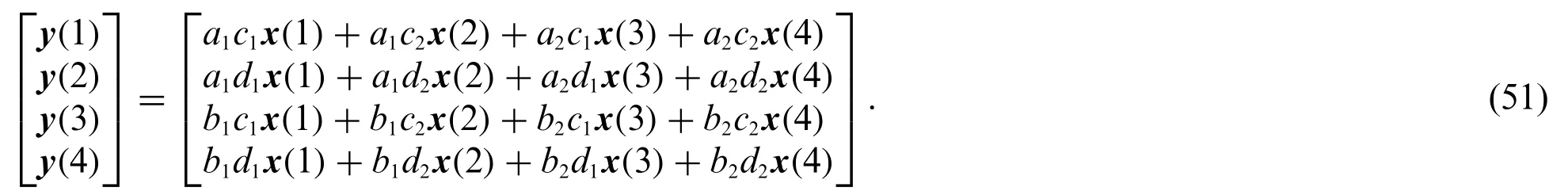
Applying Eq.(51)to cov(y2(1),y2(3))gives

cov(y2(1),y2(3))

and then Eq.(52)implies E[y2(1)y2(3)]≠E[y2(1)]E[y2(3)].

Generally,for somei≠j,E[y2(i)y2(j)]≠E[y2(i)]E[y2(j)].

Acknowledgement:The authors thank Osman Asif Malik and Stephen Becker for helpful suggestions and discussions.

Funding Statement:This work is supported by the National Natural Science Foundation of China(No.12071291),the Science and Technology Commission of Shanghai Municipality (No.20JC1414300)and the Natural Science Foundation of Shanghai(No.20ZR1436200).

Conflicts of Interest:The authors declare that they have no conflicts of interest to report regarding the present study.