A Geometrically Exact Triangular Shell Element Based on Reproducing Kernel DMS-Splines

Hanjiang Chang,Qiang Tian and Haiyan Hu

1School of Aerospace Engineering,Beijing Institute of Technology,Beijing,100081,China

2China Academy of Launch Vehicle Technology,Beijing,100076,China

ABSTRACT To model a multibody system composed of shell components,a geometrically exact Kirchhoff-Love triangular shell element is proposed.The middle surface of the shell element is described by using the DMS-splines,which can exactly represent arbitrary topology piecewise polynomial triangular surfaces.The proposed shell element employs only nodal displacement and can automatically maintain C1 continuity properties at the element boundaries.A reproducing DMS-spline kernel skill is also introduced to improve computation stability and accuracy. The proposed triangular shell element based on reproducing kernel DMS-splines can achieve an almost optimal convergent rate.Finally,the proposed shell element is validated via three static problems of shells and the dynamic simulation of a flexible multibody system undergoing both overall motions and large deformations.

KEYWORDS DMS-splines;reproducing kernel;kirchhoff-love shell;C1 continuity;multibody system dynamics

1 Introduction

The nonlinear finite shell formulation has been successfully used to study numerous problems of shell structures over the past few decades [1]. According to the classic theory of shells [2], there are mainly two kinds of shells.That is,the thick shells with a ratio of edge length to thickness less than 20 and the thin shells with such a ratio larger than 20.In general,the thick shell is described by using the Reissner-Mindlin theory with the transverse shear deformations taken into account,while the thin shell is modeled by using the Kirchhoff-Love theory without the transverse shear deformations along the thickness direction.For many shell structures in practice,such as an accurate telescope assembled by different shell patches, the high-order continuity among shell patches is required. However, it is difficult to develop a Kirchhoff-Love element withC1continuity by using the standard shape functions of Lagrange polynomials.

To reach a globally smooth and geometrically exact discretization, Hughes et al. [3] proposed the concept of the Isogeometric Analysis (IGA) in 2005. This technique has been considered as a benchmark method in the field of computational mechanics. The IGA based tensor-product Bsplines/NURBS applications [4] can be found in many fields, such as structural mechanics [5-14],fluid mechanics[15-19],and contact mechanics[20-27].In the field of multibody system dynamics,Shabana et al. [28] and Mikkola et al. [29] pointed out that the cubic B-spline curves and surfaces can be converted to the absolute nodal coordinate formulation (ANCF) for slender beam element and thin shell element without any geometric distortion.Sanborn et al.[30,31],and Lan et al.[32,33]proposed a thin beam element of rational ANCF (RANCF) with the same original CAD geometry of the cubic NURBS curves.In addition,Nada[34]proposed a plate element based on the B-spline surface in the case of large deformations.Yamashita et al.[35]comparatively studied the convergence of finite element solutions of B-spline and ANCF beam element.They found that the B-spline element and the ANCF element with same orders and continuities will lead to identical results. Based on the Integration of Computer Aided Design and Analysis (I-CAD-A) technique, three new ANCF triangular shell elements represented by Bézier triangles are proposed by Chang et al. [36], which enriches the family of ANCF elements. Again, Goyal et al. [37] and Maurin et al. [38] respectively extended the Isogeometric Euler-Bernoulli beam element and Kirchhoff-Love quadrilateral shell element to model flexible multibody dynamics.Phung-Van et al.[39]used the IGA plate to study the functionally graded piezoelectric material under thermo-electro-mechanical loads.Compared with the plate elements with traditional Lagrange interpolation, their results indicated that the accuracy and reliability for the geometrically nonlinear responses of the plate can be obtained.

Over the past few years,many IGA based Kirchhoff-Love rectangular shell elements[2,12,14,37,40,41] have been proposed. However, the application of these elements is limited because a single B-spline/NURBS patch can only represent the surfaces of rectangular topological type. In general,an arbitrary topological shell surface can be described by using the network of B-spline/NURBS patches. Nevertheless, it is difficult to enforce a certain degree of continuity between the adjacent shell patches[4].The major drawback of the B-spline/NURBS is that the gaps at intersections of shell surfaces can not be avoided.In addition,the complicated parameterization of the arbitrary topological computation domain is a time-consuming task [42]. Besides, one B-spline/NURBS patch utilizes a tensor product structure,which makes the representation of the detailed local features inefficient.In order to achieve the local refinement,the T-splines have been further incorporated into the IGA[43-46].Till now,it is still a challenge to model the complicated geometry with an arbitrary topology by T-splines,because it is not easy to obtain the linear dependent T-splines[47].In order to achieve the continuity and the local refinement in the arbitrary topological computation domain,Hughes et al.[3]pointed out that it is an opportunity for research in IGA to develop the isogeometric analysis with triangle or tetrahedron elements. Rational Bézier triangles are used for domain triangulation of complex geometries by Liu et al.[48,49],which increase the flexibility in discretization.

In fact, in the field of computer graphics and computer aided design, the DMS-splines [50](also named triangular B-splines) can be used to describe a broad class of objects with arbitrary and non-rectangular topology. The DMS-spline surfaces are able to provide an elegant and unified representation scheme for all the piecewise continuous polynomial surfaces over a planar parametric domain [51]. The other feature that makes DMS-splines attractive for surface description is their low degree. For example, aC1continuous surface can be constructed by using the quadratic DMSsplines, which have the parametric degree 2 in total. However, if the standard quadratic tensorproduct surfaces such as B-spline/NURBS surfaces are used,the parametric degree in total will be 4.Franssen et al.[52]proposed an efficient scheme to evaluate the DMS-splines in modeling the complex smooth surfaces.Qin et al.[53,54]presented the DMS-splines and rational DMS-splines to model the free form surface with non-rectangular topology.This method is based on the dynamic behavior of the model results in response to the applied forces and constraints.Pfeifle et al.[55]proposed a method to fit the DMS-spline surface by using the scattered points data,and obtained the smooth surfaces by combining the least squares method and bending energy minimization method.Furthermore,Mihalík used the DMS-splines to model the human head surface[56,57],and proposed an effective algorithm for generating the knot-net.

In general, the global continuity and local refinement surfaces can be modeled with the DMSsplines,while the DMS-splines do not perform well in computer aided engineering without adjustment[58]as a direct surface approximation based on the DMS-splines is sensitive to the placement of knots.When the knots are far from or very close to the vertices of the triangles in the parametric domain,the DMS-splines may numerically deviate from the partition of unity property,and the summation of their derivatives may not be close to zero[59].Thus,the direct use of the DMS-splines as the interpolation functions may lead to considerable errors in the approximation of the DMS-spline surfaces in the computational domain.In order to address this problem,according to the reproducing kernel element method,Sunilkumar et al.[59]proposed the reproducing kernel DMS-splines(RKDMS)to remove the unexpected errors and instability of the DMS-splines. Sunilkumar et al. [59] and Jia et al. [58]obtained the optimal convergence rate in in solving 2D linear solid problems and the partial differential equations (PDEs) based on the RKDMS, respectively. Sunilkumar et al. [60] further proposed the smooth DMS-spline finite element method and used the method to solve nearly incompressible nonlinear elasto-static problems.Sunilkumar et al.[61]also studied the wrinkled and slack of nonlinear 3D elastic membranes based on the smooth DMS-splines finite element method, and obtained satisfactory results compared with the results of the laboratory experiments. Nevertheless, it is still an open problem to establish the thin shell elements based on the RKDMS.

The objective of this study is to propose a geometrically exact Kirchhoff-Love triangle shell element based on the RKDMS.The rest of the paper is organized as follows.In Section 2,a brief review of DMS-splines is given, and the RKDMS evaluation schemes are systematically presented. Then,the geometrically exact Kirchhoff-Love triangle shell element is derived in Section 3.To compute the generalized internal force vector and the Jacobian matrix of the shell element,the derivative evaluation schemes of RKDMS are also deducted in this section.The solution strategies of the dynamic equations are presented in Section 4. Finally, in Section 5, the results of several static problems of shells are provided to validate the proposed shell element, and the dynamics of a flexible multibody system is simulated. In Section 6, the main conclusions of the study are drawn, and the future studies on this subject are outlined.

2 Reproducing Kernel DMS-Splines

The DMS-splines were originally proposed by Dahmen et al. [50] in 1992. The theoretical foundation of DMS-splines is based on the simplex splines of approximation theory[52].The simplex splines are the multivariate generalization of the univariate B-splines.In order to represent the DMSspline surface with triangular topology,the basic concept of the simplex splines are firstly revisited.

2.1 Description of the Simplex Splines

A simplex spline of degreenis a smooth, piecewise polynomial function defined by a set ofn+Ndim+1 points described by a position vector t ∈Rdimin the parametric domain.Ndimis the dimension of the parametric domain. Here, the bivariate simplex splines (Ndim=2) are considered.The knot-set V={t0,t1, ... ,tn+2}is defined as a finite set of points inR2of the parametric domain Ω.Thesen+3 points in V are called knots.A simplex spline defined over V is a piecewise polynomial of degreen.According to the work of Franssen et al.[52],a simplex splineM(p|V)of degreencan be described by a recursive equation,

where p(ξ, η) is an arbitrary point in the planar parametric domain Ω described by the orthogonal cartesian coordinate system O-ξ-η,as shown in Fig.1,and W=(w0,w1,w2)∈V is an arbitrary(nondegenerate)triangle from the knot-set V.M(p|V{wi})is a simplex spline of degreen-1 defined by the knot-set, V{wi} denotes that the knot wi,i=0, 1, 2 is removed from the kont-set V. Therefore,the simplex with degreencan be obtained by the linear combination of three simplex splines of degreen- 1. When there are only three knots in knot-set V denoted by |V|=3, the simplex splineM(p|V)=1/|det(V)|is a constant simplex.det(V)is the determinant of the three knots in the knot-set V,and it can be calculated by

where t0=(t0ξ,t0η),t1=(t1ξ,t1η),and t2=(t2ξ,t2η)are three knots in the knot-set V.λi(p|W),(i=0,1,2)are the barycentric coordinates of the point p(ξ,η)respected to the triangle W with three vertexes w0,w1,w2.As illustrated in Fig.1,the three barycentric coordinates λi(p|W)can be defined as

whereSdenotes the area of the triangle Δw0w1w2with three vertexes w0=(w0ξ,w0η),w1=(w1ξ,w1η)and w2=(w2ξ,w2η).Similarly,S0,S1,andS2respectively denote the areas of the three sub-triangles Δpw1w2,Δw0pw2and Δw0w1p.

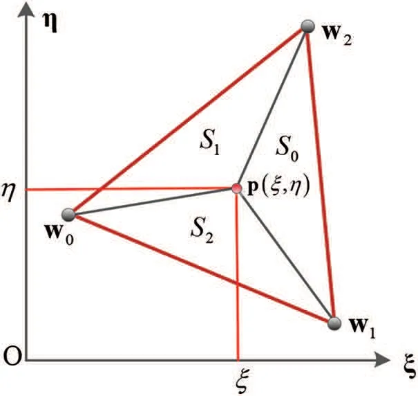
Figure 1:Schematic view of the barycentric coordinates

In Eq.(1),[V)stands for a half open convex hull,the readers can refer to the work by Farin[62]to know how to construct a half-open convex hull of a triangle. Fig.2 shows some simplex splines.Fig.2a gives a simplex spline of degree zero with three knots t0=(0.2, 0.2), t1=(0.7, 0.2), t2=(0.5,0.6), Fig.2b presents a linear simplex spline with four knots t0=(0.2, 0.2), t1=(0.6, 0.7), t2=(0.3,0.6), t3=(0.7, 0.1), and Fig.2c illustrates a quadratic simplex spline with five knots t0=(0.2, 0.2),t1=(0.6, 0.1), t2=(0.9, 0.3), t3=(0.7, 0.7) and t4=(0.4, 0.6). From Fig.2, it can be found that the constant simplex spline is discontinuous at its domain boundary, the linear spline isC0continuity and the quadratic simplex spline isC1continuity. Therefore, in order to represent the mid-surface of Kirchhoff shell element withC1continuity,we focus on the quadratic simplex spline.According to Eq.(1),the quadratic simplex spline can be calculated by the linear combination of three linear simplex splines. Similarly, the single linear simplex spline can be calculated by a similar recurrent procedure with the combination of three constant simplex splines.Fig.3 gives a schematic view of the quadratic simplex splineM(p|{t0,t1,t2,t3,t4})calculation process.

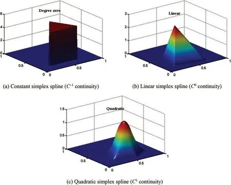
Figure 2:Simplex spline examples

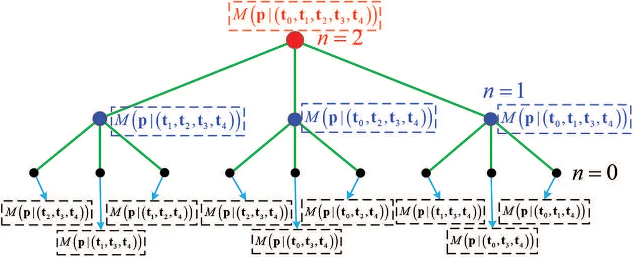
Figure 3:Tree structure of the entire calculation the quadratic simplex spline M(p|{t0,t1,t2,t3,t4})

2.2 Description of the DMS-Splines

The DMS-splines,which in fact are the weighted sum of the simplex splines,are the functions that possess the features of the global smoothness and the local supporting[51].Different from the concept of the knot-set defined in the Section 2.1,the knot-net is used to define the DMS-splines.

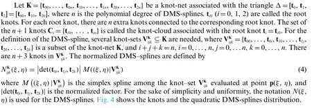
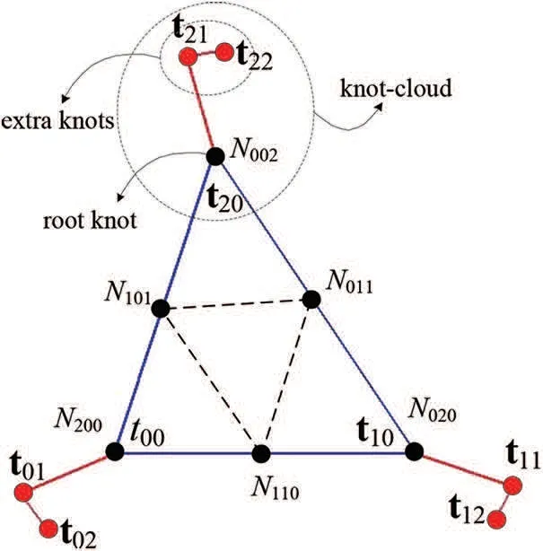
Figure 4:Distribution of DMS-splines for quadratic case with knots

A DMS-spline surface is generally composed of several surface patches with separate triangles on the parametric domain,as illustrated in Fig.5.The position of an arbitrary point on the DMS-spline surface can be expressed by

wheremis the total number of the DMS-splines,and ciis the control point of the DMS-spline surface defined in the global coordinate systemX-Y-Z.

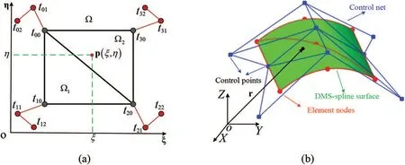
Figure 5:(a)Triangulation domain composed of two triangles.(b)Graph of the quadratic DMS-spline surface

From Fig.5,it can be found that the non-zero contributions of the particular surface patch are not only in the areas of the corresponding triangle but also in the surrounding triangles, because the DMS-splines have a larger definitional domain compared with the triangle domain composed of the three root knots ti0(i=0,1,2).This feature is the main difference from the classical methods of construction smooth triangular surfaces[62].If the non-zero contributions of the particular surface patch are only in the areas of corresponding triangle, the DMS-splines will degenerate into Bézier triangles. The interference of the DMS-spline surface patches ensures a global smoothness of the whole surface without any additional limitations on the control points. The triangulation shown in Fig.5a is composed of two triangles with one adjoining side and two shared vertices.For the quadratic DMS-spline surface,there are 12 knots and 9 control points.A quadratic DMS-spline surface for the triangulation and a control net are shown in Fig.5b. From Fig.5b, it can be seen that the control points are not located on the DMS-spline surface.

From the above analysis,it can be found that the location of the knots in the parametric domain play an important role in determining the DMS-splines. A major restriction on the position of the knot-cloud is that three knots can not be collinear [57] for a smooth surface. This is a severe task to obtain the knot-cloud over the parametric domain.In this study,the algorithm for generating the knot-net proposed by Mihalík[57]is adopted.This method considers the distance between the main knot and the extra knot as the only variable.The distance is defined as approximately 8%of the triangle shortest side in the parametric domain,and this choice is found to work well for most problems[59,60].The knot-cloud configurations based on this knot-net generation algorithm with internal and external boundaries are shown in Fig.6.

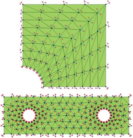
Figure 6:Knots for constructing the quadratic DMS-spline surfaces

2.3 Reproducing Kernel DMS-Splines

The DMS-splines have been proposed more than two decades.However,till now there is no robust rule or criteria to show how to construct the analysis-suitable DMS-splines.The challenge is due to the flexibilities of the DMS-splines.The performance of the DMS-splines is influenced by the uniformity of triangulation and the placement of knot clouds.From Eq.(4),although the quadratic DMS-splines areC1continuous, the DMS-splines may numerically deviate from the partition of unity property[3] and the summation of their derivatives may not be close to zero [59]. These drawbacks could account for many unexpected errors occurring in the numerical quadrature for the stiffness matrix and generalized internal force vector. In order to overcome this problem, the reproducing kernel approximation technique is adopted to improve the numerical stability and accuracy of the DMSsplines in this study.This idea is motivated by the reproducing kernel particle method[63-66],which is one of the most popular mesh-free methods.It improves the shape functions through multiplying the original shape functions by some correction terms.In IGA,this technique has been successfully applied to solve the mechanics problem with the tensor product NURBS in non-rectangular topology[67].

According to the work by Sunilkumar et al.[59],the improved approximation for the DMS-splines can be expressed as

where Φi(ξ,η)are the improved shape functions containing the correction parts.qiare the generalized coordinates located on the DMS-spline surface,as illustrated in Fig.5b.The improved shape functions can be written as

where bT(ξ, η)H(ξ-ξi, η-ηi) is the correction term for the shape functions. H(ξ-ξi, η-ηi) is a set of polynomial basisα=0,...,n, β=0,...,n. The symbolnis the order of the DMS-splines. b(ξ, η) denotes the coefficient vector of the polynomial basis for the DMSsplinesNi(ξ,η),and(ξi,ηi)are the coordinates in the parametric domain of the triangle node pointiassociated to DMS-splines. For the quadratic DMS-splines, there are six triangle nodes for each triangle including three vertexes of the triangle and three midpoints of three edges,as shown in Fig.4.And,the polynomials H,which need to be considered in the correction term,can be expressed

Considering that the improved shape functions should be satisfied the partition of unity and higher order polynomial reproducing properties,the coefficient vector b(ξ, η) in Eq.(7) can be determined by following conditions[58]

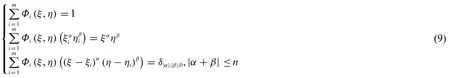
It is easy to prove that the first two equations of Eq.(9)can be a unified expression with the last equation of Eq.(9).For example,for the last equation of Eq.(9),if α=β=0,=1 can be obtained.Therefore,substituting Eq.(7)into the last equation of Eq.(9)yields

where H(0)=[1,0, ...,0]Tis a constant(n+1)×(n+1)/2 by 1 vector,and the moment matrix D is a square matrix of order(n+1)×(n+1)/2,which can be expressed by:[59]

Thus,the coefficient vector b can be obtained rapidly by solving the small-scale linear Eq.(10).Finally,substituting the coefficient vector b into Eq.(7),the improved shape functions Φi(ξ,η)yield the following implicit form:

It is should be noted that as the coefficient vector b depends on the location of the parameter(ξ,η),the detailed expressions of the improved shape functions are varied in the parameter domain.The evaluation of coefficient vector b for the quadrature points can be accomplished in the preprocessing stage of the finite element analysis,which will not decay the computational efficiency.

3 Kirchhoff-Love Shell Element Based on the RKDMS

3.1 Kinematic Description and Equilibrium Equation

According to the Kirchhoff-Love shell theory,the shell transverse shear deformation is neglected and the straight lines normal to the mid-surface will remain normal to the mid-surface after deformation.As shown in Fig.7,πzdescribes an arbitrary layer parallel to the mid-surface π of the thin shell. In the initial reference configuration, the global position of an arbitrary pointPz0(ξ1,ξ2,ζ) on the surface πzcan be expressed as[68]

where the subscript‘0’indicates the initial state,ξ1and ξ2can be regarded as the convective curvilinear coordinates of the shell,and ζ denotes the distance between the mid-surface π and the surface πz,with-h/2 ≤ζ ≤h/2,his the shell thickness.r0indicates the position vector of the corresponding pointP0(ξ1,ξ2)on the mid-surface π,which can be described by using the reproducing kernel DMS-spline surface.n0is the unit normal vector of the mid-surface π at pointP0(ξ1,ξ2).For further deformation analysis,a local curved surface coordinate frame(g0z)1-(g0z)2-(g0z)3and an element local orthogonal coordinate frame(e0z)1-(e0z)2-(e0z)3are defined at the point(ξ1,ξ2,ζ),as shown in Fig.7.The detailed definitions of(g0z)1-(g0z)2-(g0z)3and(e0z)1-(e0z)2-(e0z)3can be found in the authors’previous works[68,69].Similarly,in the current configuration of Fig.7,the coordinate frames(gz)1-(gz)2-(gz)3and(ez)1-(ez)2-(ez)3are also presented.

Figure 7:General motion of a thin shell element

According to the continuum mechanics [62], the matrix of deformation gradient F can be expressed as

where dX0denotes the infinitesimal arc segment defined in the initial reference configuration,and dx0indicates the deformed arc segment defined in the current configuration.The deformation gradient F can be decomposed with an orthogonal matrix R and a nonsingular symmetric matrix U,written as

where the right stretch tensor U can be extracted via decomposition from the deformation gradient F by separating the rigid-body rotation R,and they can be expressed as

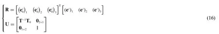
where R denotes the transformation matrix of the two local Cartesian coordinate frames(ez)1-(ez)2-(ez)3and (e0z)1-(e0z)2-(e0z)3, and the matrix T0denotes the transformation matrix from (e0z)1-(e0z)2-(e0z)3to(g0z)1-(g0z)2-(g0z)3,which can be expressed as

Similarly,in the current configuration the matrix T can be expressed as

According to continuum mechanics and the orthogonality relation between vectors (e0z)1and(e0z)2,the Green-Lagrange strain of the layer πzof the shell element can be written as

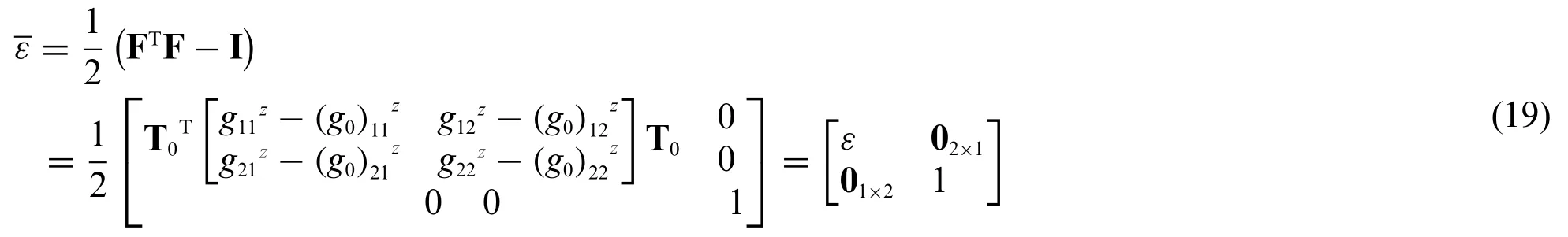
Finally,the Green-Lagrange strain tensor ε can be recast as

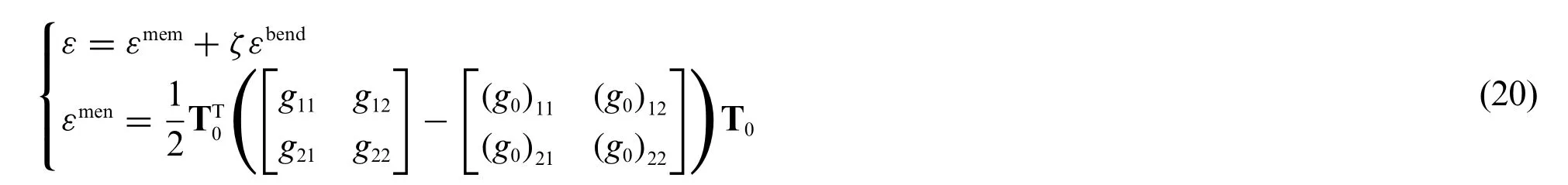
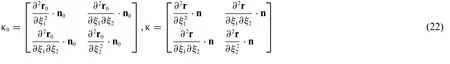
where εmemrepresents the membrane strain of the shell element,and εbenddenotes the bending strain of the shell element and can be further cast as

where

Using a St.Venant-Kirchhoff material model in order to describe an isotropic and linear elastic material,the second Piola-Kirchhoff stress tensor σscan be written in Voigt notation

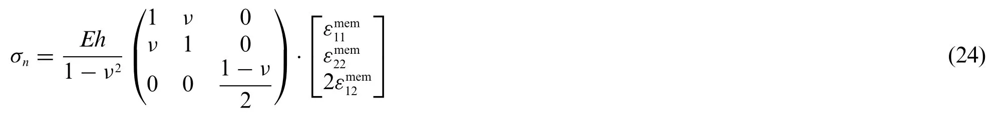
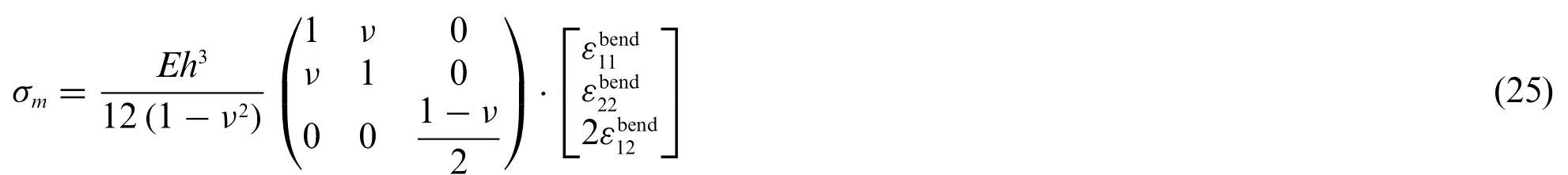
whereEis the Young’s modulus and ν is the Poisson’s ratio.ε11,ε12,and ε22are the three components of the Green-Lagrange strain tensor ε.

Substituting Eqs.(20) and (21) into (23) and integrating the Eq.(23) through the thickness direction ζ,-h/2 ≤ζ ≤h/2,the stress resultant with the membrane strains σncan be defined

and the bending strains σmcan be written as

The internal virtual work is defined by

For solving the nonlinear equation system Eq.(26),the Newton-Raphson method is used,

where Δq is the infinitesimal increment of the element generalized coordinates q.

Based on Eq.(28),the first derivative of the virtual work is the residual force vector Fr

where Fextis the external load vector and Fintis the vector of generalized internal forces,

The second derivatives of the virtual work yield the Jacobians J,which can be written as

The Jacobian matrix Jintis obtained by deriving the above term for the internal virtual work with the generalized coordinates

where the first two terms represent the material part of stiffness matrix and the latter two the geometrical part of stiffness matrix. When calculating the generalized internal force vector Fintand the Jacobian matrix Jint, the first and second derivative of the RKDMS should be involved, which will be discussed in detail in the following subsection. Besides, the numerical quadrature is applied to calculate the Jacobian matrix Jintand the generalized internal force vector Fintover each triangle parametric domainA,while the supports of the shape functions are not aligned with the integration domain[70].In order to minimize the numerical quadrature error,the triangle parametric domain is subdivided into 9 sub-triangles.In our implementation we choose 3 Gauss quadrature points in each sub-triangle for the quadratic RKDMS.

3.2 Evaluation the Derivative of the RKDMS

In order to calculate the generalized internal force vector and the Jacobian matrix deduced in the previous subsection,the first and second derivative of the reproducing kernel DMS-splines with respect to the parameter coordinates are required. According to Eq.(1), the first derivative of the DMS-splines can be calculated as follows[58]:

where ∇(·)are the derivatives of the function to the parameter coordinates ξ and η.nis the order of the DMS-splines,and the coefficientsµican be calculated by

Substituting Eq.(34)into Eq.(33),the derivative of the DMS-splines can be calculated,and the second derivative of the DMS-splines also can be calculated in the same way. The quadratic DMSsplines and their derivatives to ξ are illustrated in Figs.8 and 9,respectively.

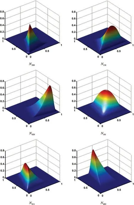
Figure 8:Schematic view of quadratic DMS-splines

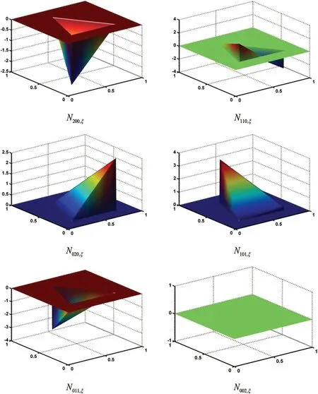
Figure 9:Schematic view of quadratic DMS-spline derivatives

From above analysis,based on the Eq.(7),the derivatives of the reproducing kernel DMS-splines Φi(ξ,η)could be calculated by

where ∇Ni(ξ, η) can been obtained by solving Eq.(33), and ∇H(ξ-ξi, η-ηi) can also be obtained by solving Eq.(8). Therefore, in Eq.(35) ∇bT(ξ, η) is the only unknown variables. The gradient of Eq.(10)can be expressed as

Obviously,∇bTcan be obtained by

Substituting Eq.(37) into Eq.(35), the derivative of the reproducing kernel DMS-splines Φi(ξ,η)can be obtained.The reproducing kernel DMS-splines and their derivatives have been constructed through Eqs.(7)and(35),respectively.The quadratic RKDMS and their derivatives to ξ are illustrated in Figs.10 and 11,respectively.In the Kirchhoff-Love shell theory,the second order derivatives of the reproducing kernel DMS-splines with respect to the parameter coordinates need to be considered to calculate the bending strain. Furthermore, the second derivatives can be calculated with the similar method.

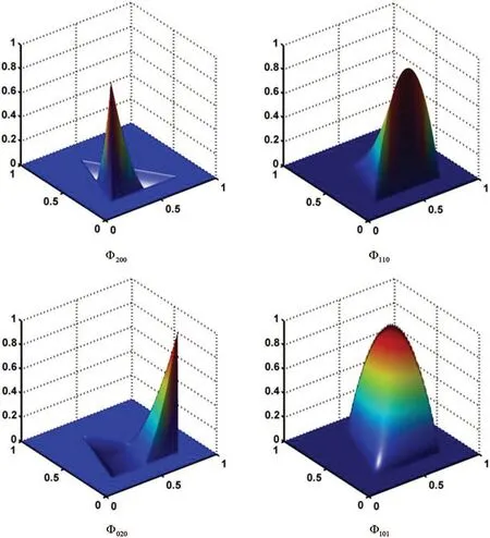
Figure 10: (Continued)

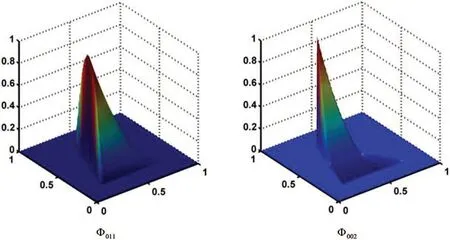
Figure 10:Schematic view of a quadratic RKDMS

Figure 11: (Continued)

Figure 11:Schematic view of the quadratic RKDMS derivatives

4 Computation Solution Strategy for Flexible Shell Multibody Systems Dynamics

According to the assembly procedure of finite elements, the dynamic equation of a constrained flexible multibody system can be expressed as a set of differential algebraic equations as follows[71]:

where M is the mass matrix of the system, Fintis the elastic force vector, φ represents the vector containing the system constraints and φqis the corresponding Jacobian with respect to the generalized coordinates q, λ is the vector of Lagrange multipliers, and Fextis the vector of external generalized forces,which can be obtained by using the principle of virtual work from Eqs.(30)and(32).

In the present study,the generalized-alpha implicit algorithm proposed by Chung et al.[72]is used to solve Eq.(38).This algorithm enables one to reach an optimal combination of accuracy at the lowfrequency range and numerical damping at the high-frequency range.Some studies[73,74]indicated that the generalized-alpha algorithm is identical to‘the three parameters optimal schemes’originally proposed by Shao et al. [75,76]. These two identical algorithms have exhibited good applicability to even tougher problems solved by Liu et al.[77-79]and Tian et al.[80]by in studying the dynamics of a flexible multibody system with clearance joints.Readers can also gain an insight into the efficient parallel computation strategy in the work by Liu et al.[79-81].

5 Case Studies and Discussions

In this section, the proposed shell element is firstly validated via three static problems of shells.Then,the validated shell element is used to study the dynamics of a flexible multibody system of shells undergoing both overall motions and large deformations.

5.1 Infinite Plate with Circular Hole under Constant in-Plane Tension

The first case study focuses on a classic linear elasto-static problem of an infinite plate with a stress-free circular hole under uniform tension,as shown in Fig.12.The structural symmetry of the problem enables one to study a quarter of the plate only.The geometric and material parameters used are:the radius of the hole isR=0.5,the edge length of the finite quarter plate isL=2,the Young’s modulus isE=105and the Poisson’s ratio is ν=0.3.

Figure 12: Infinite elastic plate with a circular hole: problem domain, boundary conditions, and material parameters

Under the Neumann boundary condition[3],the problem yields an exact solution as follows:

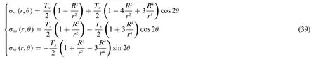
whereTx=10 is the magnitude of the applied stress for the infinite plate,(r,θ)are the polar coordinates.The traction boundary conditions are imposed on the right (x=2) and top (y=2) edges, and the symmetry boundary conditions are imposed on the left(x=0)and bottom(y=0)edges,respectively.

A comparison is made for the convergence rate of theL2norm of the stress error obtained by using the quadratic element, the Bézier triangle element [36], the DMS-splines element and the RKDMS element. Fig.13 shows the five models with different mesh sizes. Fig.14 shows theL2norm of the stress errors corresponding to the meshed models shown in Fig.13. It is obvious that the quadratic RKDMS element has the best convergence rate compared with other elements.In Tables 1-3,hdenotes the longest edge length of all the triangle elements and the DOFs stands for the degrees of freedom.It can be found that the results obtained by using the quadratic RKDMS element are much more accurate than those from other elements.As can be seen in Table 3,the convergence rate of theL2norm of the stress error for the quadratic RKDMS element is 1.82,which is close to the optimal convergence rate.However,Tables 1 and 2 show that the convergence rates of the quadratic DMS and Bezier elements are not as good as that of the quadratic RKDMS element.All the comparison results show that the reproducing kernel technique of can significantly enhance the convergence rate of a shell element.

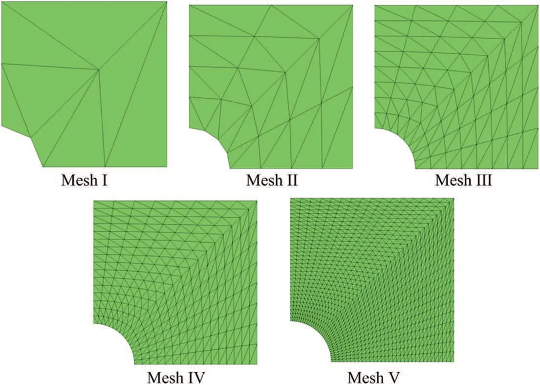
Figure 13: Infinite elastic plate with a circular hole: meshes discretization for the quadratic case employed in the error convergence study

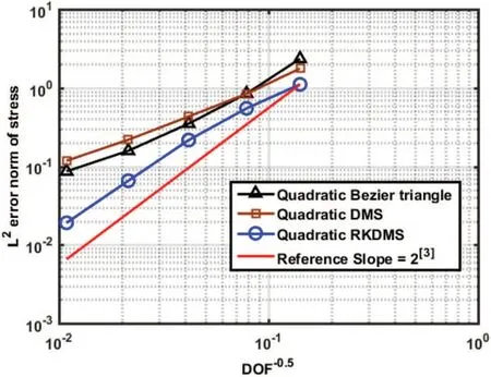
Figure 14: Convergence of the L2 norm of the stress error for quadratic Bézier triangle, quadratic DMS-splines and quadratic RKDMS with different mesh discretization

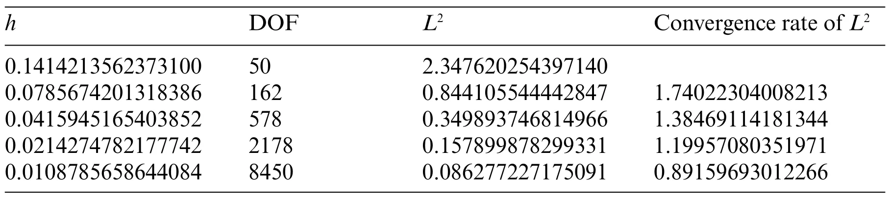
Table 1: Convergence of the L2 norm of the stress error for quadratic Bézier triangle

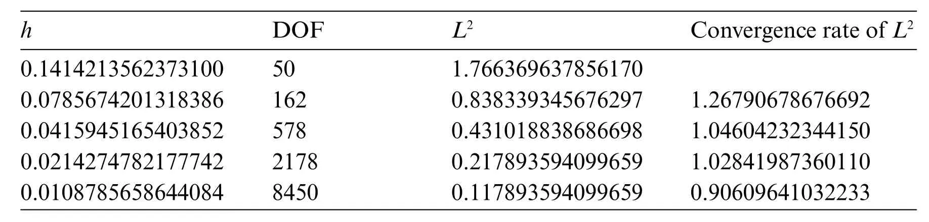
Table 2: Convergence of the L2 norm of the stress error for quadratic DMS-splines

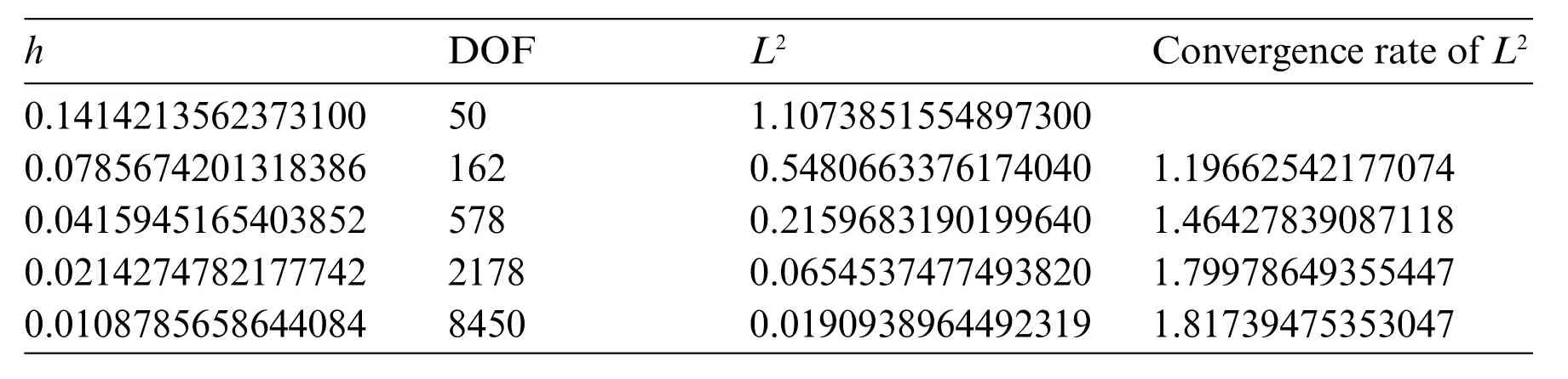
Table 3: Convergence of the L2 norm of the stress error for quadratic RKDMS

Fig.15 presents the σxxcontours for the mesh V discretized by three kinds of elements. The figure indicates that the stress contour obtained by using the RKDMS elements is smoother and more accurate than those from the Bézier element and DMS-splines element.In addition,the stress results achieved by using the RKDMS element are in a good agreement with the analytical solutions.

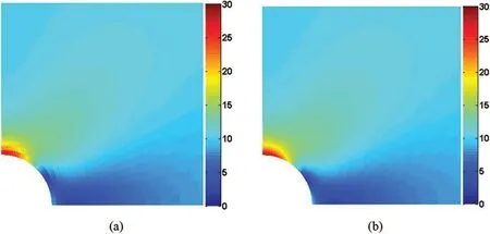
Figure 15: (Continued)

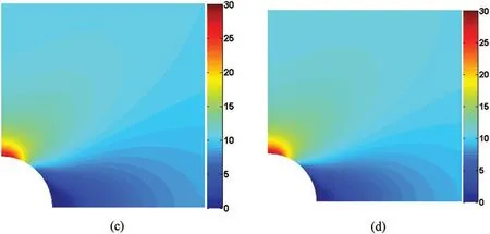
Figure 15: Contour plots of σxx for the infinite elastic plate with a circular hole for the model mesh V:(a)Quadratic Bézier triangle;(b)Quadratic DMS-splines;(c)Quadratic RKDMS;(d)Analytical solution

5.2 Nonlinear Clamped Plate under a Uniformly Distributed Load

The second case study is a square plate subject to a uniformly distributed pressure,as illustrated in Fig.16.This problem has been studied by Ubach et al.[82],Stolarski et al.[83]and Valdés et al.[84].Now,the geometric and material parameters are taken as the same in those studies.That is,the length of the plate isL=2a=20, the thickness ish=1, the Young’s modulus isE=12 and the Poisson’s ratio is ν=0.Similar to the first case study,only a quarter of the plateOMBNshould be studied.The symmetric boundary conditions are imposed along two edgesOMandON,while the other two edgesBMandBNare clamped.

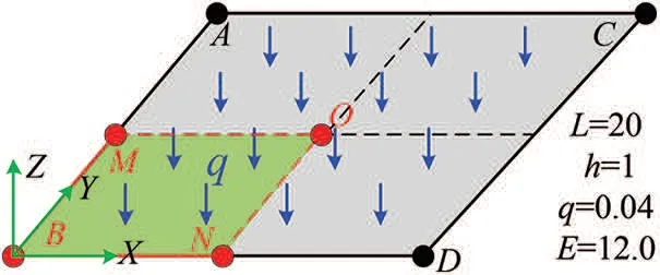
Figure 16:A nonlinear clamped plate under uniformly distributed load

Fig.17 presents three structured mesh models(Mesh I:50 elements with 121 nodes;Mesh II:200 elements with 441 nodes;Mesh III:800 elements with 1681 nodes)and one unstructured mesh model(Mesh IV:813 elements with 1702 nodes)for the plateOMBNwith quadratic RKDM elements.To study the influence of the load magnitude on the results,the transversal displacementwat the central point of the plate is normalized with respect to the thicknessh,while the uniform distributed loadqis normalized with respect toDh/a4,withD=Eh3/12.

Fig.18 gives the ‘load-displacement’ curves of the mesh models. To make a comparison, the problem is also solved by using 1600 S4R elements in the commercial software ABAQUS. Fig.18 indicates that the converged result is in a good agreement with those from ABAQUS. Besides, the results of the structured Mesh III well agree with those of the unstructured mesh IV. Fig.18 also shows the importance of geometrically nonlinear effects on large displacements compared with the linear analysis.Fig.19 gives the vertical displacement contours of the deformed models.

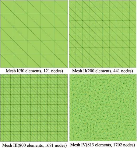
Figure 17:Different mesh models

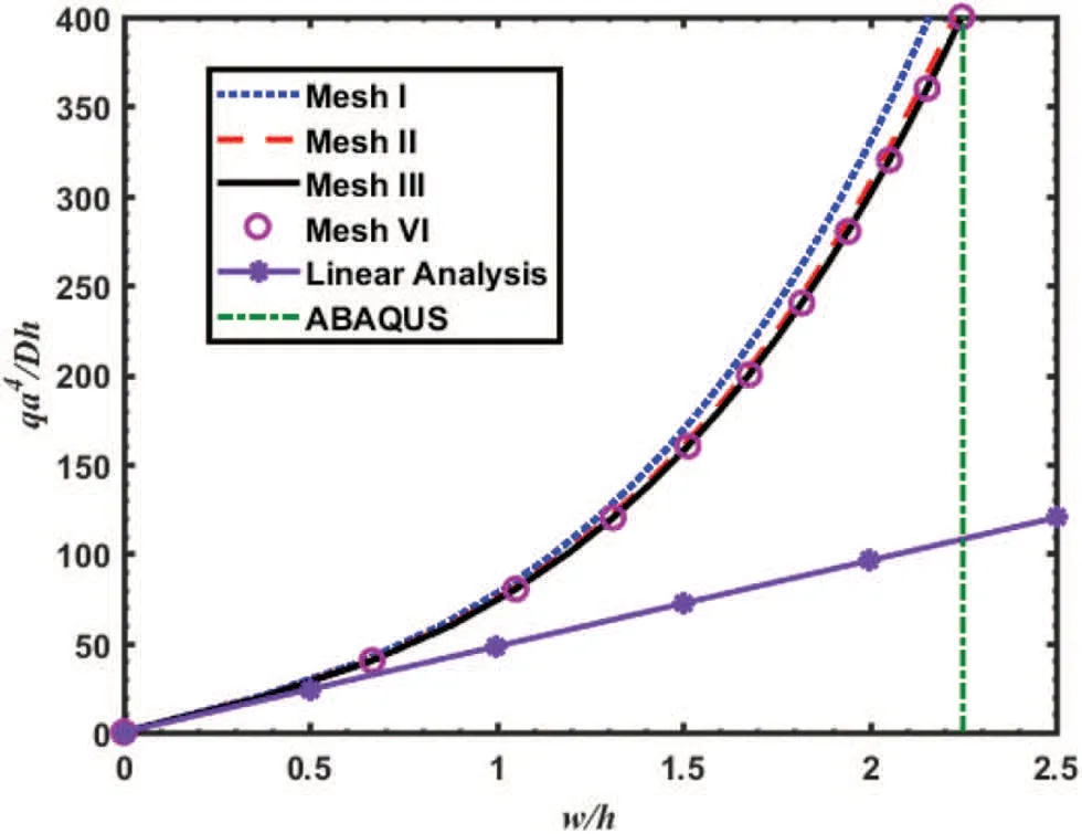
Figure 18: Load vs. center displacement of point O for the plate problem (The reference result with ABAQUS is 2.2507)

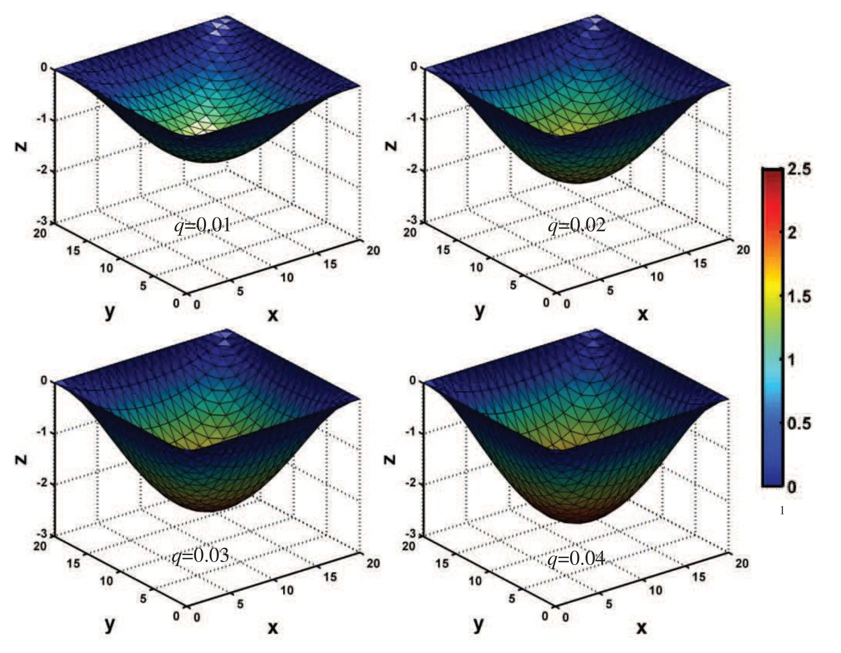
Figure 19:Vertical displacement contours and deformation configurations of models under different loads

5.3 Buckling Analysis of a Pinched Cylinder with Free Edges

This example is a popular benchmark problem in the field of finite element technology and provides a severe test for the RKDMS proposed in this paper.The same model has been studied by previous works [36,77]. As shown in the Fig.20, a free cylindrical shell is subjected to two opposite concentrated force at the midpoint of the top and bottom surface.As suggested in previous literatures,the length of the cylindrical shell,L,is set to be 10.35,and the inner radius,R,and the thickness are 4.953 and 0.094, respectively. The force applied at the shell is 40. The elastic material properties is represented by the Young’s modulus E=10.5×106and Poisson’s ratio v=0.3125.As a consequence,the results provided by this paper are compared with those preformed in previous works and the results calculated by the commercial software ABAQUS.

By taking into account the symmetry considerations,only the one upper quarter of the structure is studied. The applied load for this problem is outward relative to the shell surface, and the ends of the cylinder are free. Three meshes with different number of elements are shown in Fig.21, and the ‘load-displacement’ curves of the corresponding mesh are presented in Fig.22, whereF=40λ,0 ≤λ ≤1.The convergence mesh is composed of 29403 DOFs for the quadratic RKDMS,while the results of commercial software Abaqus with 2500 S4R elements are serveing as the reference solutions and the lifting formulation match the reference solutions well.The deformed cylinder configurations are shown in Fig.23. The deformation is not magnified, illustrating the large displacement. From the displacements of pointsBandC, it is obviously that the response of the shell has two different stages. The beginning of deformation process is dominated by bending with a large displacement.Subsequently,when the loads approximateF=20,the displacement of shell is characterized by a very stiff response.

Figure 20:Buckling analysis of a pinched cylinder with free edges:Initial configuration and material parameters

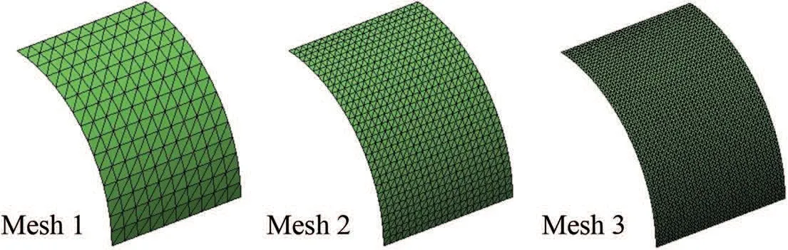
Figure 21:Thin cylindrical shell surface meshes:Meshes 1-3

Figure 22:Magnitudes of displacements at nodes A,B and C

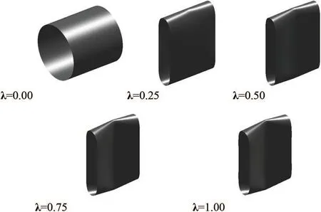
Figure 23:Deformed configurations of the cylinder under pulling forces with Mesh 3

5.4 Hemispherical Shell

The fourth case study focuses on two hemispherical shells.One has an 18°hole as shown in Fig.24 and the other does not have any hole.The two hemispherical shells have been used to validate the shell elements in many works[85,86].

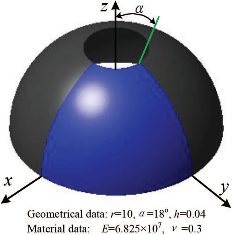
Figure 24:The problem statement of the hemispherical shell with 18°hole

For the hemispherical shell with an 18°hole at one side,the geometric and material parameters,as well as the load,are the same as those in previous literatures.That is,the radiusr=10,the thicknessh=0.04,the Young’s modulusE=6.825×107,and the Poisson’s ratio ν=0.3.Only a quarter of the shell needs to be studied because of the structural symmetry.The initial geometry(Fig.25b)is mapped from a plane rectangular reference configuration(Fig.25a)with a mesh of 4×4×2 elements via the following spherical mapping

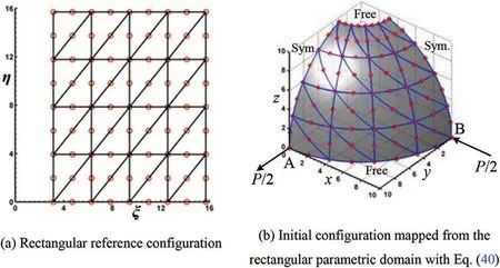
Figure 25:Hemispherical shell with 18o hole-reference and initial configurations

The displacements of pointAandBunderP=400 are shown in Table 4,where the results well agree with those obtained by using the S4R shell element in software ABAQUS,and the results look better with an increase of the element number.Besides,the deformed shape of the whole shell for the final load step is depicted in Fig.26,simultaneously the precision of the imposed symmetry conditions can be visually assessed.

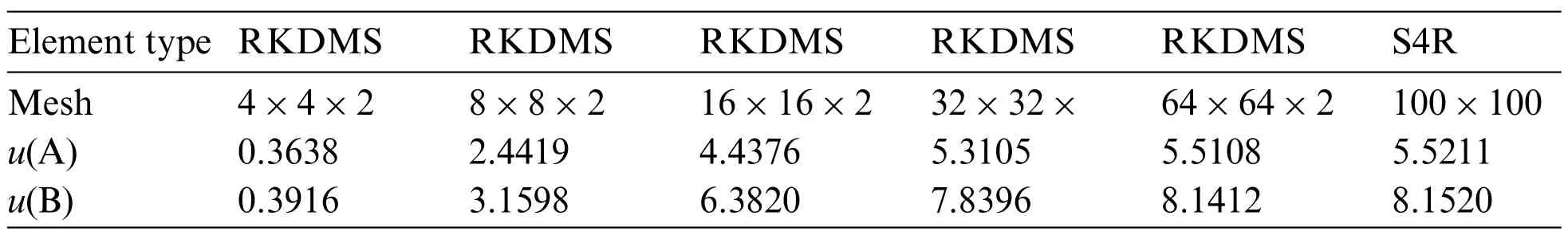
Table 4: Displacements at points A and B of the hemispherical shell with 18°hole

Figure 26:Deformed configuration of the hemispherical shell with 18°hole for the load P=400

The hemispherical shell without any hole has the same geometric and material parameters as the hemispherical shell with a hole,but is a more challenging problem.To perform the dynamic simulation by using the proposed method, an initial discretization from Fig.27a is replaced by the one from Fig.25a.The spherical mapping in Eq.(40)is still applied to the discretization from Fig.23a to build the initial configuration in Fig.27b.The alternative triangular reference configuration from Fig.27c can also be considered for the solution of the full hemispherical shell problem.The specific mapping in Eq.(41) is designed to build a complete sphere octant of the prescribed radius, see Fig.27d. The symmetric boundary conditions are imposed along the horizontal and diagonal sides of the reference domain.

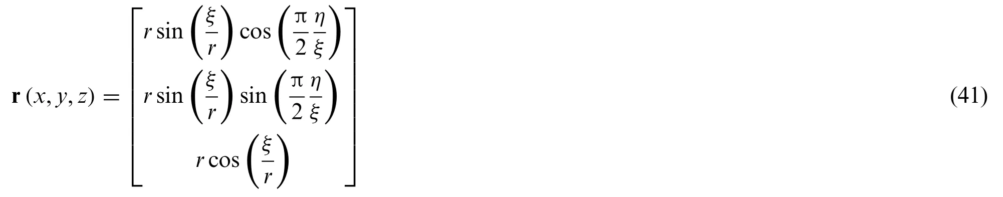
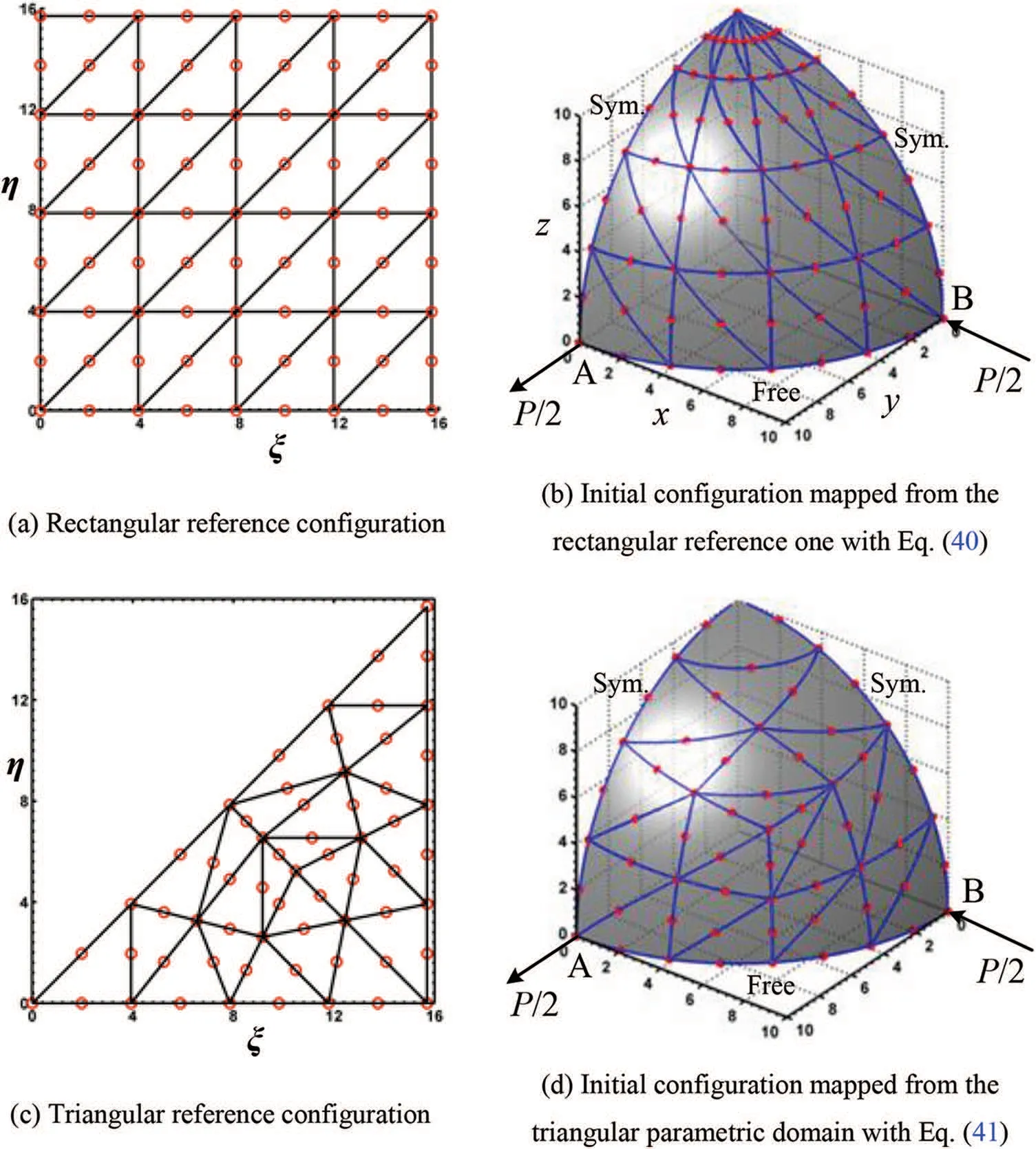
Figure 27:The hemispherical shell configurations

In order to perform a fair comparison of efficiency of these two reference configurations, the displacements of pointsAandBunderP=400 are shown in Tables 5 and 6,respectively.It is obvious that the triangular reference configuration provides better results than the rectangular one.The results based on the proposed formulation are in a good agreement with those simulated with dense S4R element in ABAQUS.Fig.28 shows the deformed configuration of the hemispherical shell under the loadP=400.

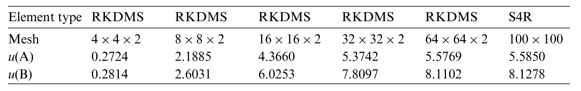
Table 5: Displacements at points A and B of the full hemispherical shell mapping with rectangular reference configuration

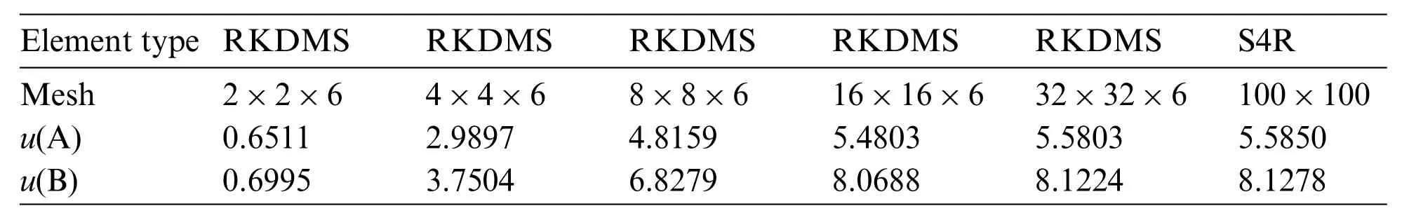
Table 6: Displacements at points A and B of the full hemispherical shell mapping with triangular reference configuration

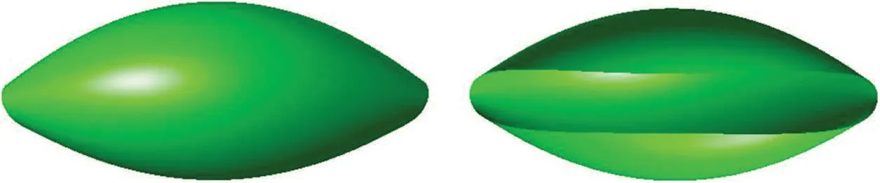
Figure 28:Deformed configuration of the full hemispherical shell for the finial load P=400

5.5 Dynamics of a Double Pendulum Composed of Two Octant Spherical Shells

The final case study is to simulate the dynamics of a double pendulum composed of two identical octant spherical shells,as shown in Fig.29.The initial geometry of an octant spherical shell is mapped from a plane triangular reference configuration with Eq.(41).The Young’s modulus of the material is 6.825×107Pa,and the material density is 7810 kg/m3,and the Poisson’s ratio is 0.3.The geometry properties are radius of 0.5 m and thickness of 0.01 m, and the gravitational acceleration is chosen as 9.81 m/s2. The four corner pointsA,B CandDare initially located on the horizontal planex-ywith the concave side upward for one shell and the concave side downward for the other shell. The corner pointAis restrained to the ground via a spherical joint,which prevent the corner pointAfrom any translation displacement,but does not limit any rotation.The two shells are connected with two spherical joints at pointsBandC,as shown in Fig.29.

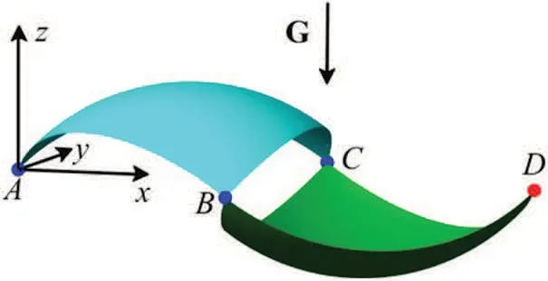
Figure 29:Initial configuration of the double pendulum

An objective of this case study is to check the influence of the number of the proposed thin shell elements on the system dynamics.As shown in Fig.30,the difference of the system displacement at pointDin z-direction becomes smaller and smaller with an increase of the number of finite elements.Fig.30 indicates that the mesh of 8×8×12 shell elements is enough to give convergent results. To ensure the correctness of the simulation dynamics,it is helpful to check the total energy of the system,as shown in Fig.31,with respect to time,whereT,VandUare kinetic energy,deformation energy and potential energy of the system,respectively.As the double pendulum is a conservative system,the total energy should be a constant all the time.Fig.31 presents the energy conservation holds true for the model,with a mesh of 8×8×12 shell elements.Fig.32 shows the dynamic configuration of the system at four specific moments.

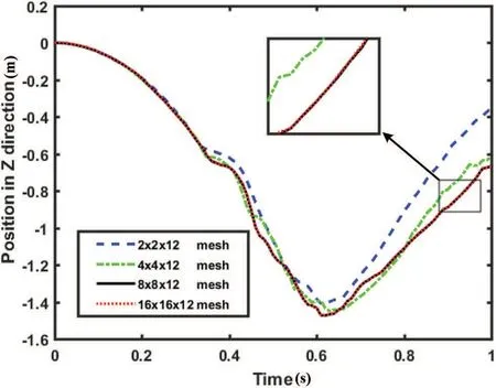
Figure 30:The motion of point D in z-direction of the double pendulum with different mesh densities

Figure 31:Energy balance of the free falling double pendulum

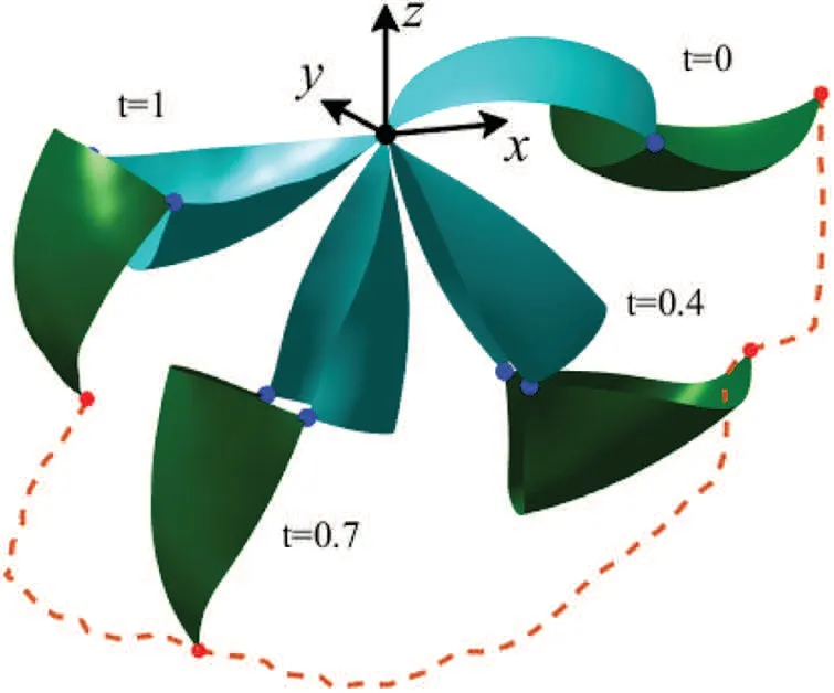
Figure 32:Dynamic deformed configurations of the double pendulum(8×8×12 mesh)

6 Concluding Remarks

The paper presents how to establish a geometrically exact Kirchhoff-Love shell element via the reproducing kernel DMS-splines for the dynamics of multibody systems. The procedure is general and can be applied to thin shell systems with complex topology.The reproducing kernel DMS-splines surface has shown to be well-suited for modeling Kirchhoff-Love shell elements because it is easy to reach theC1continuity.The number of degrees of freedom of the proposed shell elements is quite low compared with the traditional thin shell elements based on the standard shape functions of Lagrange,because each node of the shell element has only three translational degrees of freedom.In addition,the reproducing kernel approximation of the DMS-splines ensures the computation stability and accuracy of the proposed shell element, and improves the convergence rate of the proposed formulation.The paper demonstrates the efficacy of the proposed formulation via four static problems of shells,as well as the dynamic simulation of a flexible double pendulum composed of shells undergoing both overall motion and large deformation.As a part of future work,it is possible to extend the technique to more complicated systems based on tetrahedral meshes and the trivariate DMS-splines.

Funding Statement:This work was supported in part by the National Natural Science Foundations of China under Grants 11290151,11672034 and 11902363.

Conflicts of Interest:The authors declare that they have no conflicts of interest to report regarding the present study.