
2D Minimum Compliance Topology Optimization Based on a Region Partitioning Strategy
2023-02-17 03:13ChongWangTongxingZuoHaitaoHanQianglongWangHanZhangandZhenyuLiu
Chong Wang,Tongxing Zuo,2,Haitao Han,2,Qianglong Wang,2,Han Zhang and Zhenyu Liu,*
1Changchun Institute of Optics,Fine Mechanics and Physics(CIOMP),Chinese Academy of Sciences,Changchun,130000,China
2School of Optoelectronics,University of Chinese Academy of Science,Beijing,100049,China
ABSTRACT This paper presents an extended sequential element rejection and admission(SERA)topology optimization method with a region partitioning strategy. Based on the partitioning of a design domain into solid regions and weak regions,the proposed optimization method sequentially implements finite element analysis(FEA)in these regions.After standard FEA in the solid regions,the boundary displacement of the weak regions is constrained using the numerical solution of the solid regions as Dirichlet boundary conditions.This treatment can alleviate the negative effect of the material interpolation model of the topology optimization method in the weak regions,such as the condition number of the structural global stiffness matrix.For optimization,in which the forward problem requires nonlinear structural analysis,a linear solver can be applied in weak regions to avoid numerical singularities caused by the over-deformed mesh.To enhance the robustness of the proposed method,the nonmanifold point and island are identified and handled separately.The performance of the proposed method is verified by three 2D minimum compliance examples.
KEYWORDS Topology optimization;region partition;nonmanifold point;matrix conditional number;geometric nonlinearity
1 Introduction
Topology optimization aims to obtain the optimal material distribution with prescribed constraints in a fixed domain.Since the pioneering work of Bendsoe et al.[1],many methods have been proposed to achieve topology optimization,such as density-based methods[2],boundary evolutionbased methods [3,4], differential equation-driven methods [5-7] and geometric component methods[8-10]. Density-based methods can be further divided into continuous variable methods [11] and discrete variable methods[12,13].We refer the readers to references[14,15]for the fast progress and successful application of topology optimization.
In an early discrete variable method,the evolutionary structural optimization(ESO)method as proposed by Xie et al. [12], ineffective or inefficient materials were eliminated directly to achieve optimization. This method has high computational efficiency but cannot add material. To remedy this deficiency,various versions of bidirectional evolutionary structural optimization(BESO)methods were proposed to allow material removal and addition.The earliest version of BESO[16,17]allowed new elements to grow around elements with high stresses. Yang et al. [18,19] proposed evaluating the strain energy of the elements to be added by linear extrapolation of the displacement field.Huang et al.[20,21]proposed using mesh-independent filters to evaluate the sensitivities of standby additive elements. In the above methods, all the elements in the holes are directly removed, so these methods are called hard-kill type methods.
In hard-kill type methods,the ability to change topology is usually related to the material introduction strategies[22].As an alternative to this,soft-kill type methods were proposed in which the holes are mimicked by weak material.In this type of method,the sensitivities of the elements in holes can be calculated directly without extrapolating from the information of the solid elements.The existing softkill type methods include the sequential element admissions and rejections method(SERA)proposed by Rozvany et al. [23-25], the penalty-based BESO method proposed by Huang et al. [26] and the topology optimization method with sequential integer programming proposed by Liang et al.[13,27],etc.The weak material introduced by soft-kill type methods is similar to the density lower limit of the SIMP material model.They both retain elements in holes for calculating sensitivities,thus providing a standard for adding material.
Introducing a weak material has been proven to be very successful in solving static small deformation problems and has become a standard model in topology optimization.To ensure smooth access to the optimal solution,the physical property of the weak material must be controlled within a reasonable range.If the value is too large,the stiffness provided by it cannot be ignored,which may lead to an overly rigid performance evaluation.If too small,the condition number of the structural stiffness matrix becomes worse,and large numerical errors may occur in the results.Therefore,the condition number is usually selected as 10-3.In addition,in some specific optimization problems,a weak material may cause numerical instability or even incorrect results. For example, when a structure has a large deformation,excessive mesh deformation may occur in weak regions,which leads to nonconvergence of the Newton-Raphson iteration[28,29].In the topology optimization of a buckling structure,pseudo bucking modes may appear in the weak regions[30], which adversely affects the effectiveness of the results.
The hard-kill type methods and some other methods that remove the elements in the holes can avoid the problems caused by weak materials[21,31-33].However,as mentioned above,these methods generally decide the introduction of material through the extrapolation of information(displacement,strain energy or sensitivity,etc.)from solid elements.Eliminating the negative effects caused by weak material in soft-kill type methods is the focus of this paper.
From the perspective of model consistency, the physical model and finite element (FE) model are consistent in the hard-kill type methods, but the FE model of the soft-kill type methods is an approximate model from the physical model. If the inconsistencies between the two models are eliminated,it is possible to solve the above problems in the framework of soft-kill type methods.
In SERA, the concepts of real material and virtual material are introduced to distinguish the elements (it should be noted that the real material and virtual material here correspond to the solid and weak material mentioned above.To avoid confusion,only the concepts of solid and weak materials are retained in the next content.The sensitivities of solid elements and weak material elements(weak elements)are ranked,and two thresholds are selected to determine the elements to be removed or to be added.This method indirectly divides the design domain into solid regions and weak regions but does not further identify them.The design domain is still regarded as a whole for FEA in this method.Tong et al.[34]proposed a moving ISO-surface threshold method(MIST),in which the topological boundaries are determined by a response function threshold based on physical properties, so the design domain can also be divided into two parts.Wang et al.[35]proposed an energy interpolation framework to address geometric nonlinear optimization problems. In this framework, the elastic energy densities of solid regions and weak regions are obtained by interpolating the elastic energy density of nonlinear theory and linear theory,respectively,thus avoiding the numerical instability of weak regions under finite deformation.Bruns[36]proposed an algorithm to allow void material to be replaced by zero density elements.The algorithm can reject weak materials,but the SD/SVD approach they used is computationally expensive.Nguyen et al.[37]preconditioned the stiffness matrix to avoid ill-conditioned problems caused by the 0 density lower bound.Li et al.[38]proposed a meshless moving morphable component(ML-MMC)method,in which the structural analysis was carried out only on the solid regions,avoiding the intervention of weak materials.
Based on the characteristics of the above methods,a topology optimization method with a region partitioning strategy is proposed in this paper.The method is implemented based on SERA.The FEA is carried out regionally.To avoid the influence of weak material on the result of solid regions,FEA of solid regions is carried out first, where the weak elements are eliminated temporarily in this step.When the FEA of the solid regions is completed, FEA of the weak regions is performed with the displacement solution of solid regions as the Dirichlet boundary conditions(Fig.1).When optimizing structures under finite deformation,linear theory and nonlinear theory can be applied to the two types of regions separately to avoid numerical instability.
In the implementation,two special structural features,nonmanifold points and islands,may arise in solid regions after region segmentation.These two structural features might cause instability in the numerical solution of the displacement via FEA.We introduce concepts and algorithms in graphics to recognize and solve them:the nonmanifold points are identified by an undirected graph and treated by the minimum volume filling (MVF) algorithm and minimum sensitivity filling (MSF) algorithm[39]; the islands are identified by the fire-burning method (FBM) [40,41] and treated together with weak regions in the FEA.The solution to the above cases can improve the robustness of the proposed algorithm.

Figure 1: Schematic diagram of the original SERA model and the proposed model: (a) the original SERA model:the design domain is solved as a whole;(b)the proposed model:the design domain is solved for both the solid regions and weak regions simultaneously
The rest of the paper is arranged as follows:the topology optimization algorithm with a region partition strategy is detailed in Section 2. In Section 3, the nonmanifold point and island are introduced and solved.In Section 4,several geometric linear and geometric nonlinear numerical examples are executed to verify the feasibility of the proposed algorithm.Section 5 provides the conclusions.
2 Methodology
In SERA,solid regions and weak regions can be distinguished by densities of elements.To avoid the negative effects of weak regions on solid regions,the FEAs for the two types of regions are carried out in sequence.The optimization formula is as follows:
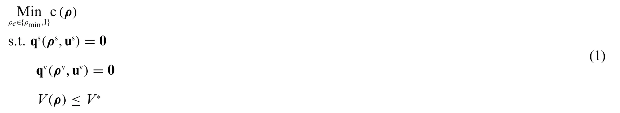
where the superscript s represents solid regions and the superscript v represents the weak regions;ρis the design variable vector andρeis its elementwise component; c is the objective function to be optimized; qs(ρs,us)=0 is the equilibrium equation of solid regions, whereρsand usare the design variable vector and state variable vector of solid regions,respectively;qv(ρv,uv)=0 is the equilibrium equation of weak regions,whereρvand uvare the design variable vector and state variable vector of weak regions, respectively;Vis the volume of material used andV*is the upper limit of allowable volume.
The only difference between the Eq.(1)and classic optimization formula is that the former has two equilibrium equations and must be solved sequentially.
2.1 Finite Element Analysis
In the proposed method,the FEA of solid regions is prioritized.Weak elements are temporarily removed in this step. When FEA of the solid regions is completed, FEA of the weak regions is performed with the displacement solution of solid regions as the Dirichlet boundary conditions.The FEA procedure is shown in Fig.2.
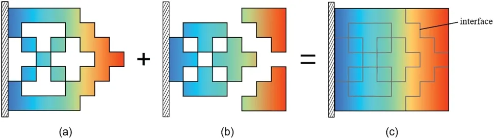
Figure 2: The FEA in the proposed method: (a) solving the displacement field of solid regions; (b)solving the displacement field of weak regions;(c)union of the displacement fields of the two types of regions
Since the element densities can only be one orρmin,the elements and corresponding node degrees of freedom(DOFs)in the solid regions and weak regions can be obtained according to the ordering rules of DOFs.Then,we can establish FE formulae of solid regions and weak regions.When considering the static small deformation problem,the FE formula of solid regions is as follows:

where Ksis the global stiffness matrix of the solid regions and fsis the load vector of the solid regions.The boundary conditions between the solid regions and the weak regions are zero Newman boundaries.Compared with the original FE model,this model removes weak elements.
In regard to the finite deformation problem,the nonlinear FE formula must be considered:

where r is the residual force;psis the external load vector of the solid regions;and fsis the load vector of the internal nodes in the solid regions at equilibrium,and its expression is as follows:

whereMsis the set of solid elements; Ceis a matrix that transforms the modal force vector of the element to the globally nodal force vector;and feis the nodal force vector of the element.
The most frequently applied scheme for solving nonlinear systems is the Newton-Raphson algorithm.It is based on a Taylor series development of Eq.(3)at a known state

where the parameter λ denotes the load level for which the solution has to be determined;DrΔukcharacterizes the directional derivative of r atand the vectorδis the residuum of the Tayler series.More details about the Newton-Raphson scheme can be found in the literature[42].
After the displacement vector usis obtained by solving Eqs.(2) or (5), we need to solve the displacement vector uv. To ensure the stability of the analysis, it can be solved simply by the linear FE formula.
In the FE model of weak regions,Dirichlet boundary conditions are imposed on the interface to maintain the continuity of the displacement field.The implementation process is as follows:first,the components of the displacement vector usneed to be rearranged.The DOFs of noninterface nodes are placed in the front as uss,and the DOFs of interface nodes are placed in the back as uc.The rearranged displacement vectoris as follows:

The global stiffness matrix, displacement vector and load vector of the weak regions are also divided into two parts according to the noninterface nodes and the interface nodes.The updated FE formula is:

where Kvvis the stiffness matrix assembled by DOFs of noninterface nodes in weak regions and Kccis the stiffness matrix assembled by DOFs of interface nodes. Kvcand Kcvare the coupling stiffness matrices,and they are symmetric.
Since uchas been obtained by Eq.(6),it can be moved to the right,and Eq.(7)can be rearranged:

When the load-independent design problem is considered, the weak regions usually have no external load so that fvis a zero vector.Eq.(8)can be simplified as follows:

The displacement vector uvis obtained by solving Eq.(9).
2.2 Sensitivity Number
In the case of small deformation problems,the sensitivity numberαeof an element that determines the element to be added or removed has been derived by Alonso et al.[43]:

where ueis the element displacement vector andΔKeis the variation in the elemental stiffness matrix.Since the densities of elements can only be one orρmin, the sensitivity values have the following two forms:

When addressing small deformation problems, according to Huang et al. [21], the structural compliance can be replaced by an incremental form. The sensitivity number of theith element is defined as

It should be noted that the sensitivity numbers in Eqs.(11) and (12) are both expressed by the element strain energy(or its negative value).However,this expression has different meanings for linear and nonlinear structures.For an elastoplastic structure,it denotes the total elastic and plastic strain energies,while for a linear structure,it is only for the elastic strain energy.

ΔVcan be limited to a definite value by adjusting the two thresholds.One can refer to reference[43]for more details about material iteration.
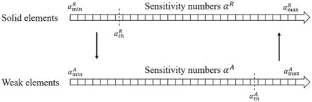
Figure 3:Material variation determined by two sensitivity thresholds
The above strategies can effectively avoid the adverse effects caused by weak elements and maintain the integrity of sensitivities. However, in the execution process, structural instability may occur due to some special structural features. To ensure the robustness of the algorithm, these structural features must be solved.
3 Nonmanifold Points and Islands
After regional partitioning,there are two structural features that may cause numerical instability:nonmanifold points and islands. They must be addressed to prevent system ill conditioning. In this section,we introduce some strategies to identify and address them.
3.1 Nonmanifold Points
Hinged elements often appear in solid regions when material is almost removed (Fig.4). These structures are usually unstable. In computational geometry, such one-point connected structures belong to nonmanifold structures,and the point is named the nonmanifold point.A more common form of nonmanifold point in topology optimization is the checkerboard pattern.The checkerboard pattern is not expected due to its overestimated stiffness and difficulty in manufacturing[44].Poulsen[45]proposed a simple and implicit scheme based on a structural grid to prevent checkerboard patterns and one-node hinges. However, we need direct control to ensure that these situations are avoided in each iteration.
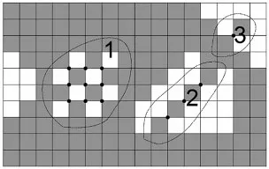
Figure 4:The structural features consisting of nonmanifold points:1 is the checkerboard pattern;2 is a hinged rod;3 is a hinged element
3.1.1 Definition of Nonmanifold Point
It is necessary to introduce the concept of a 2D manifold to describe nonmanifold points.A surface is a 2D manifold if it has the following characteristics:(1)Every point on the surface of an object has a sufficiently small neighborhood isomorphic to the disk on the plane;(2)If the surface is unclosed(it has boundaries), every point on the boundaries must have a sufficiently small neighborhood isomorphic to the half disk in the plane. Since it is impossible to describe each point on a surface by computer, the conditions identifying that a surface is a 2D manifold are represented by vertices,edges and faces of the discrete grid:(1)each edge can only be shared by two faces;(2)the edges and faces adjacent to each vertex can form one ring around it.For example,there are three points in Fig.5.The setSvi(i=1,2,3)contains all edges and faces adjacent to vertex vi.IfSvican form more than two rings topologically isomorphic to a disk,vertex vi is a nonmanifold point.According to this,v1 and v2 are manifold points;v3 is a nonmanifold point.
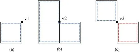
Figure 5:Manifold point and nonmanifold point:(a-b)the points v1 and v2 are manifold points;(c)the point v3 is a nonmanifold point
3.1.2 Identification of Nonmanifold Point
As the design domain is discretized by a structured rectangular mesh,the nonmanifold point is presented in only one form:adjacent elements of the vertex contain two diagonally distributed solid elements and two diagonally distributed weak elements. The procedure of identifying nonmanifold points is as follows and the flow chart is as shown in Fig.6.
(1) Create the vertex setΦ=whereis the vertex set of the solid elementiandNSis the number of solid elements.
(2) Calculate the vertex set A={x|xappears twice inΦ}.
(4) Calculate the vertex set B={x|xappears four times inΨ}.
(5) Calculate the nonmanifold point setΛ=A ∩B.
The strategy to accommodate nonmanifold point is converting the weak elements adjacent to the nonmanifold point into solid elements, as shown in Fig.7. In theory, the problem can be solved by addressing each nonmanifold point in turn, but when the nonmanifold points appear continuously in the horizontal or vertical direction (checkboard pattern), many nonessential solid elements may be introduced that severely affect the volume and the objective.To minimize this adverse effect,two algorithms are introduced to determine how to introduce solid elements.
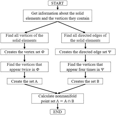
Figure 6:Flow chart of nonmanifold point identification
3.1.3 Two Algorithms to Accommodate Nonmanifold Points
Structures consisting of nonmanifold points can be divided into two categories:hinged structures and checkerboard patterns.Since the adjacent weak elements have no intersection in hinged structures,converting any of the surrounding weak elements can address the problem(Fig.7a).For the checkerboard pattern,one of the most common methods is using filtering techniques on element densities or sensitivities.Poulsen[45]proposed a framework with implicit constraints to reject nonmanifold points.Han et al.[40]suppressed the checkerboard pattern by identifying and filling a single weak element.
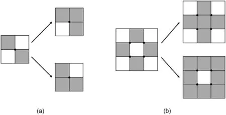
Figure 7:Nonmanifold points are rejected by converting weak elements to solid elements:(a)rejection of a single nonmanifold point;(b)rejection of multiple adjacent nonmanifold points
To reduce the disturbance to the volume and the objective, we introduced two algorithms to address nonmanifold points: the minimum volume filling algorithm (MVF) and the minimum sensitivity filling algorithm (MSF). The MVF requires filling a minimum number of solid elements to reject all nonmanifold points,and the MSF requires that the elements that are filled have the least impact on the objective.
The concept of an undirected graph is introduced to implement the above two algorithms. The graphG=G(V,E)can represent a topology consisting of solid elements in whichVis the vertex set ofGandEis the edge set ofG.If the verticesx,y∈Vare adjacent vertices,x→y∈Eis a directed edge ofGin whichxis the starting vertex andyis the ending vertex.Since the direction of the edge is not of concern to us,x→yandy→xcan be regarded as equivalent,and such graphs are called undirected graphs(also called symmetric graphs).
The undirected graphG(V,E)of the checkerboard pattern in Fig.8a can be constructed as an example: since it is known that a nonmanifold point has two adjacent weak elements, these two elements can be regarded as the vertices of the graphG. The nonmanifold point is their edge. The checkerboard pattern can be converted to the undirected graphG.The gray dots belong to the vertex setV,and the dotted lines belong to the edge setE,as shown in Fig.8b.

Figure 8: The process of addressing checkerboard patterns based on the MVF: (a) a checkerboard pattern;(b)the undirected graph G;(c)minimum covered vertex set;(d)the result after filling elements
(1) Minimum Volume Filling(MVF)
The MVF can be transformed into minimum point set coverage,which means that each edge in the undirected graph must be associated with at least one of its vertices. In graph theory, the minimum point set covering is equal to the maximum matching so that the Hungarian algorithm [39] can be used to solve the problem.The gray dots in Fig.8c are the minimum covering point set obtained by the algorithm.The result of the MVF is shown in Fig.8d by covering the weak elements corresponding to the gray dots into solid elements.
(2) Minimum Sensitivity Filling(MSF)
The MSF can be transformed into minimum point set coverage with weight in the undirected graph. In the algorithm, the sensitivity values of the weak elements adjacent to each nonmanifold point are added to the vertices of the undirected graph as weights.The minimum point set coverage with weight requires that every edge in the weighted undirected graph is associated with at least one vertex and the sum of the weights of these vertices is minimum.
As shown in Fig.9, the two algorithms are verified by two structures. The structure in Fig.9a has only one hinge,and the structure in Fig.9d has a checkerboard pattern.Figs.9b and 9e show the results of the MVF.Figs.9c and 9f show the results of the MSF.
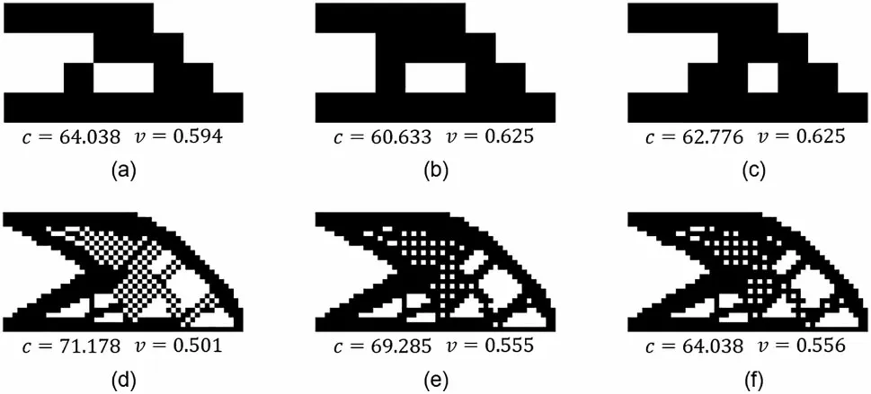
Figure 9:The two structures removing nonmanifold points by the MVF and MSF:(a)and(d)are two structures containing nonmanifold points;(b)and(e)are the results obtained by the MVF;(c)and(f)are the results obtained by the MSF
In Fig.9a,there is only one nonmanifold point,so introducing a weak element can solve it.In this case,the MVF randomly selects a weak element to fill,but the MSF selects the element with the lowest sensitivity value. In Fig.9d, many solid elements need to be introduced to solve the checkerboard pattern so that the material and objective function values will be significantly increased. The result shows that the MVF strategy requires less material, and the MSF strategy leads to less disturbance of the objective value. In summary, the MVF strategy is more suitable for handling checkerboard patterns,and the MSF strategy is more suitable for discontinued hinged structures.It should be noted that if the number of filling elements is too large in the optimization iteration,the convergence may be adversely affected. Therefore, filtering technology is still used in the following examples to suppress the checkerboard pattern.
3.2 Islands
In SERA,the initial structure is usually made entirely of solid elements.In the early optimization process, solid elements are gradually transformed into weak elements. This may lead to a situation in which some solid elements are completely separated from the main structure, forming an island(Fig.10). In the original SERA method, an island is surrounded by weak elements that have low stiffness to support it so that the island can be constrained to a certain extent and the condition number is not too large to affect the stability of the numerical calculation.However,in the proposed method,the solid regions are analyzed without weak materials. The island is free of any constraints, which adversely affects the numerical stability.

Figure 10:A structure with two islands
To accommodate islands,we need to identify them first.The recognition of the nonmanifold point mentioned above is the recognition of elements,while an island is a region composed of an uncertain number of elements.Although the domain is divided in SERA,the numbers of solid regions and weak regions are still unknown.We introduce the fire-burning method[40]to group solid material by regions,and then the boundary conditions are used to identify whether a certain solid region is an island.Since an island has no effect on the structure stiffness,we group it into weak regions for FEA.
3.2.1 Adjacent Matrix
To realize the fire-burning method,the adjacent relation of the elements must be calculated first.The concept of a graph is still used to explain here. For the graphG=G(V,E)composed of solid elements,an adjacent matrix is used to describe the adjacency relationship of elements.
The graphGis made up of solid elements, which are numbered as 1,2,...,|V|. The adjacency matrixAof graphGis a|V|-dimensional square matrix,andaijis the component of matrixA:

whereEis the set of all undirected edges.
Fig.11 shows the process of obtaining the adjacency matrix from a structure. The structure in Fig.11a consists of six solid elements. Fig.11b is converted to an undirected graphG, where each element represents a vertex ofG.If two elements are adjacent,they are connected by a black line.It should be noted that the elements may be connected by a single node or an edge,both of which indicate that the elements are adjacent.Fig.11c shows the adjacency matrixAofG.

Figure 11: Schematic diagram of adjacency matrix calculation: (a) A structure consisting of six elements.(b)Graph G with 6 vertices and 9 edges.(c)The adjacency matrix of G
For a structured grid,the coding rules of elements and their nodes are generally fixed and regular.For example,the simplest coding method is to encode from top to bottom and from left to right.We can evaluate whether the two elements are adjacent by evaluating whether there is a common node between the two elements,and the adjacency matrix of the elements can be established by this information.
3.2.2 Fire-Burning Method
The process of the fire-burning method is as follows:
(1) Determine an element as the initial burning point;
(2) Search the adjacent untraversed elements with the same density as the current burning points;these elements are regarded as the new burning points.
(3) Iterate Step 2 until there are no more qualified elements around the current burning points.All the elements in the current region can be found by the iteration.Fig.12 graphically depicts the process of Step 2 and Step 3.
(4) Determine an untraversed element as a new burning point,and repeat Steps 2 and 3.
(5) Once there are no untraversed elements in the design domain, the process ends, and all the regions have been found.
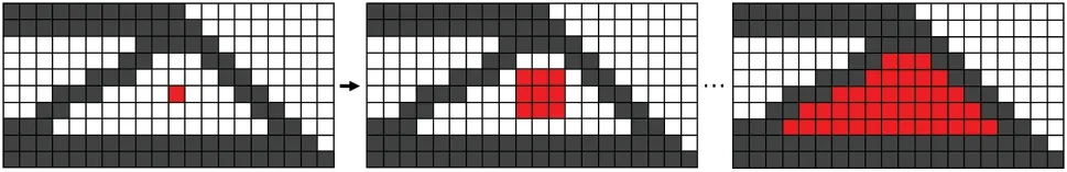
Figure 12:The process of the fire-burning method for finding a region
3.2.3 Identification and Processing of Island
Since all the regions have been found,we can determine whether a region is an island by evaluating whether there are constrained points or load points in the region.Considering little contribution to the objective function and adverse effects on the numerical stability,we group islands into weak regions for FEA.
4 Numerical Examples and Discussion
In this section,the concept of a conditional number is introduced to measure the ill conditioning of a system,and three examples are performed to verify the effectiveness of the proposed method.The first one is the short beam example;the second one is the C-shape plate example[46];the third one is the cantilever beam.All the materials in the examples are isotropic,and the material constants used are elastic modulusE=1.0 and Poisson’s ratioν=0.3.
4.1 Condition Number
The condition number of a matrix is a well-known measure of ill conditioning.For ann×nmatrix K,its condition number is:

where||·||is any matrix norm.If the matrix K is singular,we usually regard the condition number as infinite[47].
When considering the static small deformation problem,the design domain is discretized by the FE mesh,and the governing equation can be expressed by a linear equation:

where u and f are the displacement vector and the load vector,respectively,and K is the global stiffness matrix that is assembled by element stiffness matrices.
In SERA,the element stiffness matrix is expressed as follows:

whereρe=1 orρminmeans that the element is a solid element or a weak element and K0is the stiffness matrix of the solid element. It is easy to evaluate from Eqs.(15)-(17) that the condition number of K is related to the ratio of the maximum and minimum elemental density in the design domain. By convention, the density of the solid element is usually set to one. If the density of the weak element decreases,the condition number of the corresponding stiffness matrix will increase.
A simple example can illustrate this. Fig.13 shows an optimal structural topology of the short beam example. The density of the solid element is one, and the density of the weak element varies from 10-9to 10-30. The condition number of the global stiffness matrix changes as Fig.14 shows.According to the curve,the logarithm of the weak elemental density is proportional to the logarithm of the condition number of K.
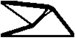
Figure 13:A structure consisting of solid materials and weak materials
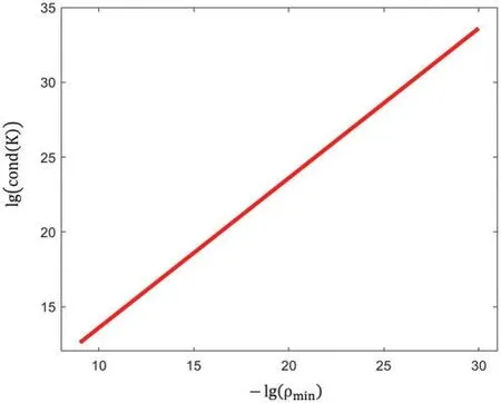
Figure 14:The curve of the condition number changing with the density of the weak elements
Since the condition number of the global stiffness matrix is a direct parameter to measure numerical stability,it can be seen from the above that two cases can lead to ill-conditioned systems:
(1) An extremely small ratio of the minimum and maximum densities.
(2) Local unstable structures.
The method proposed in Section 2 can completely solve the first case. The second case can be solved by the strategies introduced in Section 3.
4.2 Short Beam
The load and support conditions of the short beam example are shown in Fig.14. The design domain is discretized by 100×50 rectangular elements.The upper limit of the volume fraction is 0.3,and the filter radius is 0.04.
In SERA, the optimal structure can usually be obtained faster by deleting materials than by adding materials. Therefore, the initial structures in the subsequent examples are all composed of solid elements.In the first half of the optimization process,the solid elements are gradually rejected until the volume constraint is met,and then the same amounts of solid elements and weak elements are increased or decreased until convergence.

Figure 15:The design domain and boundary conditions for the cantilever beam:(a)The load is applied to the lower right corner.(b)The load is applied to the midpoint of the right boundary
In this example,four values,10-9,10-18,10-27,and 10-36,are selected as the design valuesρminof the weak elements,and the original SERA method is also conducted for comparison.The iteration curves in Figs.16 and 17 show that the order of the condition numbers almost increases inversely with the decrease inρmin,which confirms the conclusion in Section 4.1.The iteration path also changes asρminchanges.Occasionally,the condition number or objective function will increase dramatically in a step(shown in Figs.16c,16d and 17b-17d),which may greatly affect the iterative process and the optimal topology. Fig.17 shows the structural topology and displacement field in the abnormal step. There are nonmanifold points and islands in the position framed by the dotted lines in Figs.18a and 18c and abnormally large displacement values in the corresponding positions in Figs.18b and 18d.According to Figs.16e-16h and 17e-17h,after solving the nonmanifold points and islands,the condition number can be controlled from 104to 107by the proposed method and is not affected byρmin.
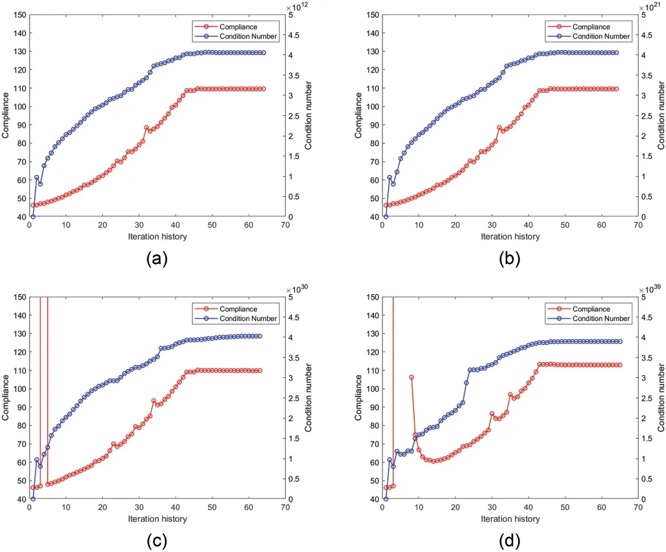
Figure 16: (Continued)
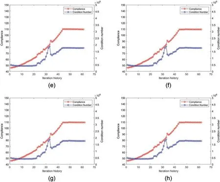
Figure 16:Iteration history of the model in Fig.15a:(a)-(d)are the iteration histories with the four densities of weak elements conducted by the original SERA;(e)-(h)are the iteration histories with the four densities of weak elements conducted by the proposed method
Figs.19-22 show the optimal topologies and corresponding objective values. In summary, the optimal results obtained by the original SERA method are affected byρmin.Onceρmindrops to 10-36,the optimal topology changes prominently.Figs.17 and 19 show that the optimal topologies are almost unchanged asρminvaries. Theoretically, the proposed method allowsρminto be arbitrarily decreased with no effect on the optimization.
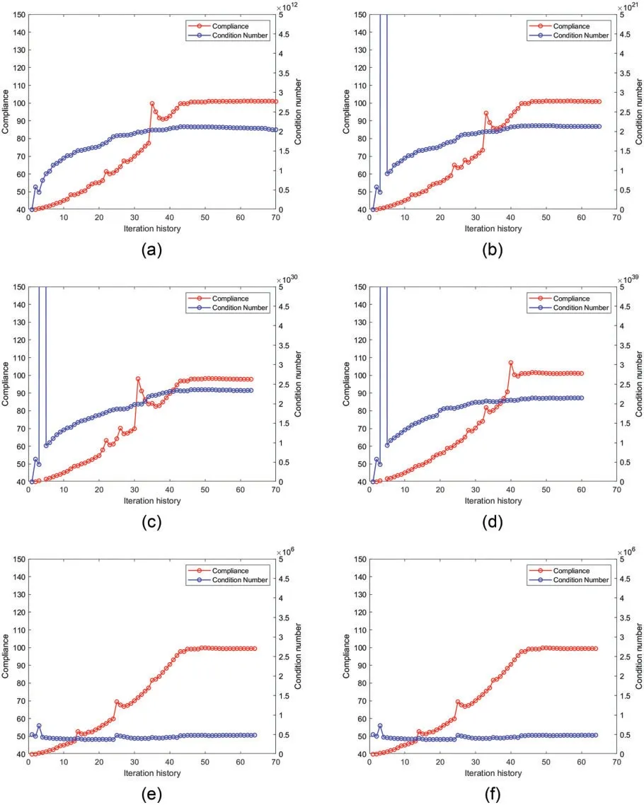
Figure 17: (Continued)
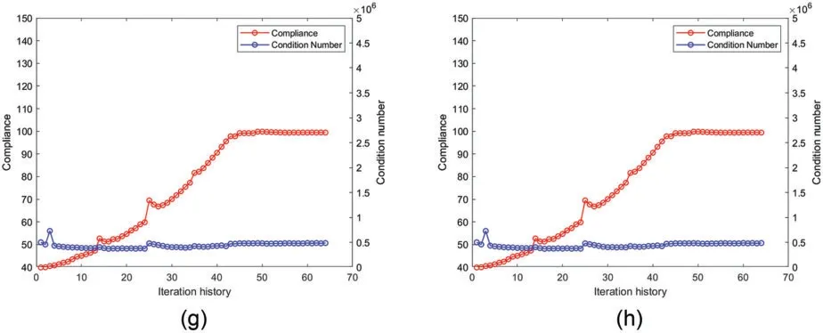
Figure 17:Iteration history of the design model in Fig.15b:(a)-(d)are the iteration histories with the four densities of weak elements obtained by the original SERA;(e)-(h)are the iteration histories with the four densities of weak elements obtained by the proposed method
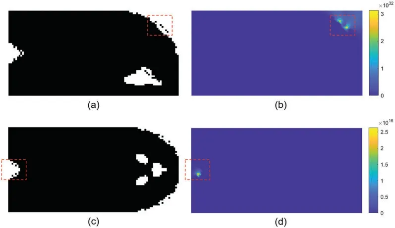
Figure 18:Structural topology and displacement field causing abnormal iteration:(a)and(b)correspond to the abnormal iteration step in Figs.16c and 16d; (c) and (d) correspond to the abnormal iteration step in Figs.17b-17d
To verify the computational efficiency of the proposed method,the computational time is counted.The original SERA consumed 9.8 and 18.4 s for computing the two examples in Fig.15;the proposed method consumed 18.0 and 23.2 s for computing the two examples.Therefore,the proposed method is less efficient than the original SERA. From Fig.23, the time consumed by the proposed method in each iteration has a large oscillation, while in the original method, the time consumed in each iteration is relatively stable. It is well known that the most time-consuming process in optimization iteration is FEA. Since the number of elements in the two methods is the same, the time consumed by FEA is basically fixed.However,there is another time-consuming process in the proposed method:nonmanifold point processing. Since nonmanifold points do not appear at every step, nonmanifold point processing is also not performed at every step, which is the reason for the oscillation of the time-consumption curve.

Figure 19: Optimal results of the design model in Fig.15a with the four densities of weak elements obtained by the original SERA

Figure 20: Optimal results of the design model in Fig.15a with the four densities of weak elements obtained by the proposed method
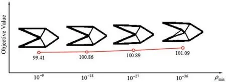
Figure 21: Optimal results of the design model in Fig.15b with the four densities of weak elements obtained by the original SERA
In this example,we also verify the stability of the proposed method under different mesh densities.Three mesh densities are considered:1)coarse,consisting of 100×50 rectangular elements;2)medium,consisting of 200×100 rectangular elements;3)fine,consisting of 300×150 rectangular elements.The loading position is shown in Fig.15a.The design value of the weak material is 10-36.The results for the three cases are shown in Fig.24.
The optimal structural topologies are almost the same for the three mesh densities. Only the boundary smoothness and the size of local holes are slightly different. Therefore, the robustness of the proposed method is not affected by the mesh density. However, there is another factor to consider as the mesh density increases: in the proposed method, the nonmanifold point processing is time-consuming. Once the elements increase, the nonmanifold points may increase, which will reduce computational efficiency. To adapt to large-scale computation, we consider how to improve the efficiency of nonmanifold point processing in future work.
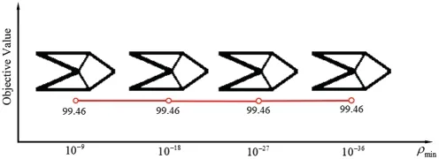
Figure 22: Optimal results of the design model in Fig.15b with the four densities of weak elements obtained by the proposed method
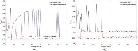
Figure 23:Time consumption curves of the short beam examples:(a)Fig.15a.(b)Fig.15b
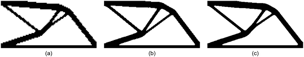
Figure 24:Short beam design for different mesh densities:(a)coarse;(b)medium;(c)fine mesh
4.3 C-Shape Plate
To verify the effectiveness of the proposed method for solving excessive mesh deformation under finite deformation, we considered an example proposed by Yoon et al. [46] shown in Fig.25. The design domain is discretized by 60×60 rectangular elements, and the concentrated forcesf1= 0.02 andf2=0.03 are loaded.The elastic modulusEof solid is one,and Poisson’s ratioνis 0.3.The design value of weak materialρminis 10-9.
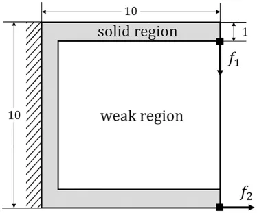
Figure 25:The design domain and boundary conditions for the C-shaped plate
For better comparison,we analyzed the structure for the following three options:(1)geometric linearity or geometric nonlinearity;(2)inclusion or exclusion of weak regions;and(3)with or without a region partition strategy.The results are shown in Fig.26.The corresponding settings and convergence for Figs.26a-26e are shown in Table 1.
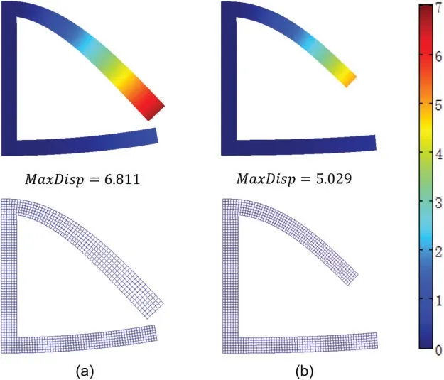
Figure 26: (Continued)
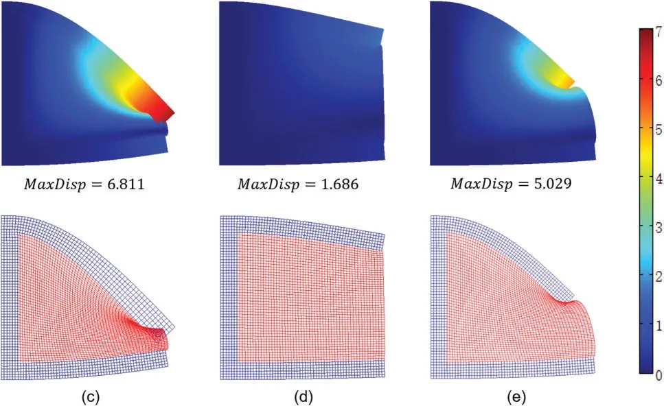
Figure 26:The scalar displacement field and deformed mesh of the C-shaped plate
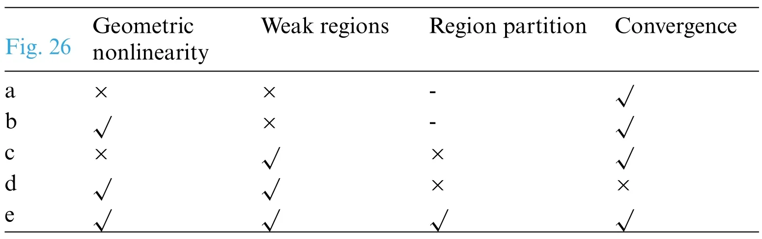
Table 1: Corresponding settings and convergence for all the results in Fig.26
When no weak region is included(Figs.26a and 26b),convergence can be achieved by a geometric linear or geometric nonlinear model.However,the maximum deformation of the former is larger than that of the latter. In addition, the rods on the upper side of the structure in Fig.26a have become significantly thicker,which is obviously unreasonable.When considering weak regions,the result of the solid regions remains the same under the geometric linear model(Fig.26c).However,in the geometric nonlinear model,the analysis process does not converge due to excessive mesh deformation(Fig.26d).After adopting region recognition,nonlinear theory and linear theory are applied to the solid regions and weak regions,respectively.As shown in Figs.26b and 26e,the results are exactly the same in the solid regions,which illustrates that the proposed method guarantees that excessive mesh deformation in the weak regions has no influence on nonlinear analysis so that convergence can be achieved.
Now, we apply the topology optimization method with a region partitioning strategy to this problem.The design domain and boundary conditions are still consistent with the model in Fig.25.The filter radius r=0.25.The volume fraction constraint is 0.28.Two initial structures(Figs.27a and 27c)are tested for optimization:in one,the design area is completely covered by solid elements with a volume fraction of one;the other is the same as the model in Fig.25,with a volume fraction of 0.28.
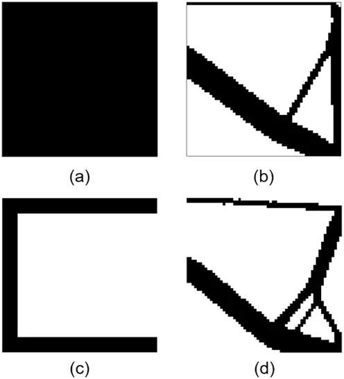
Figure 27:The optimal structures of the C-shaped plate obtained from two initial structures
As shown in Figs.27b and 27d, there are some differences in the optimal structures. The first optimal structure is identical to that obtained by Lahuerta et al.[48].The second one,which is close to the first one,is significantly worse.The reason is that the second initial structure is much different from the optimal structure and falls into a local solution. However, under the first initial structure,there is no excessive deformation in the optimization process, and nonconvergence caused by mesh distortion did not occur.To verify the proposed algorithm,the second initial structure is optimized,and the mesh deformation is captured during the optimization process,as shown in Fig.28.Although excessive mesh deformation exists in the first three steps, the optimization iteration is not adversely affected.
4.4 Cantilever Beam
The design domain and boundary condition of the cantilever beam are shown in Fig.29. The design domain is discretized by 120×30 rectangular elements. The magnitudes of the concentrated load are 0.0002,0.0005,0.0007 and 0.001.The initial volume fraction is 1.0,and the volume fraction constraint is 0.5.The design valueρminof the weak material is 10-9,and the filter radiusris 0.014.
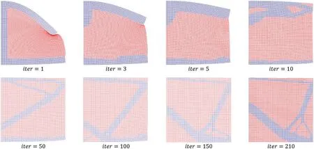
Figure 28: Deformed mesh in iteration: blue elements are solid elements; red elements are weak elements
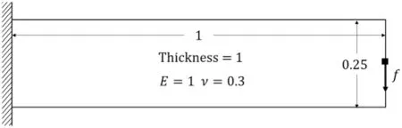
Figure 29:The design domain and boundary condition for the cantilever beam
In this example, we verify the difference in optimization results under geometric linear and geometric nonlinear assumptions based on a region partitioning strategy.The effects of different loads on the topology optimization results are examined simultaneously.The results are shown in Fig.30.On the first two lines in Fig.30,we compare the optimal structures and objective values for different loads in linear and nonlinear solutions and obtained the following conclusions:(1)As expected,under the assumption of geometric linearity,the value of concentrated force does not affect the optimal topology;(2) Under the assumption of geometric nonlinearity, the optimal topology varies substantially with the load value. When the load value is very large, its result is notably different from the geometric linear solution.(3)The objective function values in geometric linear solutions and geometric nonlinear solutions are different. When the load valuefis 0.001, the objective value of the geometric linear solution is only 17%of that of the geometric nonlinear solution.
The third line in Fig.30 shows the final deformation mesh of the geometric nonlinear solution.When the load is 0.001,the weak elements around the loading point are clearly excessively deformed(Fig.31).Due to the introduction of the region partitioning strategy,the weak regions are solved by a linear algorithm so that nonconvergence does not occur and the optimal structure can be obtained.
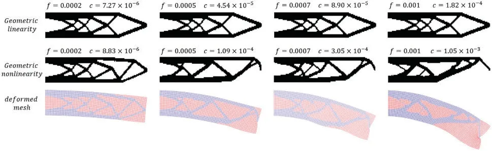
Figure 30:Optimized structure and deformed mesh for different loads
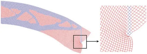
Figure 31:Excessive deformation of weak elements
5 Conclusions
Numerical instability problems caused by a material interpolation model in the weak region are considered in this paper. A topology optimization model with geometrical region partitioning and the corresponding FEA procedure is proposed. Numerical strategies to identify nonmanifold points and island structures are discussed,and numerical instability during the optimization procedure can be alleviated by properly addressing the nonmanifold points.Numerical examples illustrate that the proposed method can solve the ill-conditioned matrix problem in FEA and nonconvergence phenomena caused by excessive mesh deformation in finite deformation.The region partition strategy proposed in this paper can be implemented from SERA to other topology optimization methods,such as the SIMP method and boundary evolution type method.
Funding Statement:This work was supported by the National Science Foundation of China (Grant No.51675506).
Conflicts of Interest:The authors declare that they have no conflicts of interest to report regarding the present study.
 Computer Modeling In Engineering&Sciences2023年7期
- Computer Modeling In Engineering&Sciences的其它文章
- Edge Intelligence with Distributed Processing of DNNs:A Survey
- Turbulent Kinetic Energy of Flow during Inhale and Exhale to Characterize the Severity of Obstructive Sleep Apnea Patient
- The Effects of the Particle Size Ratio on the Behaviors of Binary Granular Materials
- A Novel Light Weight CNN Framework Integrated with Marine Predator Optimization for the Assessment of Tear Film-Lipid Layer Patterns
- Implementation of Rapid Code Transformation Process Using Deep Learning Approaches
- A New Hybrid Hierarchical Parallel Algorithm to Enhance the Performance of Large-Scale Structural Analysis Based on Heterogeneous Multicore Clusters