Numerical Simulation of the Fractional-Order Lorenz Chaotic Systems with Caputo Fractional Derivative

Dandan Dai,Xiaoyu Li,Zhiyuan Li,Wei Zhang and Yulan Wang,⋆

1School of Physics and Electronic Information Engineering,Jining Normal University,Jining,012000,China

2Department of Mathematics,Inner Mongolia University of Technology,Hohhot,010051,China

3Institute of Economics and Management,Jining Normal University,Jining,012000,China

ABSTRACT Although some numerical methods of the fractional-order chaotic systems have been announced,high-precision numerical methods have always been the direction that researchers strive to pursue.Based on this problem,this paper introduces a high-precision numerical approach.Some complex dynamic behavior of fractional-order Lorenz chaotic systems are shown by using the present method.We observe some novel dynamic behavior in numerical experiments which are unlike any that have been previously discovered in numerical experiments or theoretical studies.We investigate the influence of α1,α2,α3 on the numerical solution of fractional-order Lorenz chaotic systems.The simulation results of integer order are in good agreement with those of other methods.The simulation results of numerical experiments demonstrate the effectiveness of the present method.

KEYWORDS Novel complex dynamic behavior;numerical simulation;fractional-order lorenz chaotic systems;high-precision

1 Introduction

In 1963,Edward Lorenz discovered a mathematical model for atmospheric convection.This model is also known as Lorenz chaotic system.The Lorenz system is widely used in electric circuits,forward osmosis and chemical reactions.In recent years,people have studied the chaotic behavior in the fractional dynamic system and found that the fractional dynamic system has unique properties that the integer dynamic system does not have.Therefore,the numerical simulation of fractional chaotic system is very important.In this paper,we simulate the fractional-order Lorenz chaotic dynamical systems[1–6]is as

with the initial conditions

The solutions of the fractional-order Lorenz chaotic dynamical systems are very hard to obtain analytically,and researchers,therefore,rely on numerical methods to provide an approximate solution that could be used for prediction.In the last decades,several numerical methods have been proposed.In [1],based on the qualitative theory,the authors investigated the existence and uniqueness of solutions for a class of fractional-order Lorenz chaotic systems (1).In [2],compared the dynamical regimes of fractional-order systems with dynamical regimes of the corresponding standard systems.In[3],Complex dynamics with interesting characteristics were presented by means of phase portraits,the largest Lyapunov exponent and bifurcation diagrams.In [4–6],the authors gave a dynamic analysis of a fractional-order Lorenz chaotic system.Although some numerical and analytical methods of the FDEs have been announced,such as spectral method [7–11],reproducing kernel method[12–19],homotopy perturbation method[20–23],high-precision numerical approach[24–27],and so on numerical and analytical methods[28–36].These researchers all say their own approach can accurately simulate chaotic systems.In fact,since chaotic systems have no exact solution,researchers do not know which method is more accurate.For the numerical simulation of chaotic systems,it is necessary to use numerical methods to study the long time properties of solutions of the fractional order chaotic systems.This paper introduces a high-precision numerical method [24–27] for solving system (1).Some complex dynamic behavior of the fractional-order Lorenz chaotic systems are discovered by using the present numerical approach.We observe some novel dynamic behavior in numerical simulations which are unlike any that have been previously discovered in numerical simulations or theoretical studies.The simulation results of numerical experiments demonstrate the effectiveness of the present method.

Fractal and fractional calculus[37–48]have been widely concerned.In the last three decades,there have existed many inequivalent definitions[49–51]of fractional derivatives.The most famous of these definitions that have been widely popularized in the world of fractional calculus is Riemann-Liouville fractional definition,Grünwald-Letnikov fractional derivative(GLFD)and Caputo fractional derivative definition.

Definition 1.1.Riemann-Liouville fractional derivative of orderαof a functiony(t)aboutton the interval(t0,t)is defined as

Definition 1.2.Caputo fractional derivative of orderαof a functiony(t)∈Cn[t0,t]aboutton the interval(t0,t)is defined as

Definition 1.3.The Grünwald-Letnikov fractional derivative ofα-order on the interval(t0,t) is defined as

where

Therefore,theα-order Grünwald-Letnikov derivative in Eq.(4)is transformed into the following form:

Using Newton’s binomial theorem,we know

We can proof the following form:

(1−z)αis called 1-order generating function ofα-order Grünwald-Letnikov derivative on the interval(t0,t).

Theorem 1.4.Iff(t)is continuous and differentiable of ordern−1 on the interval(t0,t),andf (n)(t)is integrable,then Grünwald-Letnikov derivative can be written in the following integral form:

and,the Grünwald-Letnikov derivative,Riemann-Liouville derivative and Caputo derivative have the following relationship:

Proof1.For the proof,please refer to[49].

From Theorem(1.4),it follows that,ify(j)(t0)=0,j=0,1,...,n−1,then(t).If existsj,such thaty(j)(t0)/=0,j=0,1,...,n−1,we use Taylor form,let(t)=y(t)−.For convenience of expression,we denote

2 Numerical Approach

In[24–27],in order to obtain hig her precision,author given the construction method of generating function for arbitraryp,and then give a recursive method of fractional derivative and integral based on the generating function.

Definition 2.1.Ap-order polynomial function is defined as

Theorem 2.2.Theporder polynomial functiongp(z)could be written as

wheregkis the solutions of the following equation[24–27]:

Proof 2.It can be seen from Eqs.(13)and(14)

Substitutingz=1 into Eq.(16),there is

Multiply both ends of Eq.(16)byzand find the first derivative ofz,then

Then substitutez=1 into Eq.(18),then there is

Multiply both ends of Eq.(16)byz,and then find the first derivative ofz

Substitutingz=1 into Eq.(19),we can derive

Repeating the above process,the following equation can be established:

The matrix form of the equation is formula(15),which is proved by the theorem.

Definition 2.3.Ihep-order generating functiongαp(z)ofα-order Grünwald-Letnikov derivative is defined as

Theorem 2.4.If the generating functiongαp(z)can be written as

where the subsequent coefficientω(α,p)kcan be recursively calculated by the following formula[24–27]:

Proof 3.Letz=0 in Eq.(20),then it can be proved=gα0.Rewritten Eq.(20),it can be seen that

where,ifk <0,then=0.Find the first derivative ofzon both sides of Eq.(23),it can be concluded that

Both sides of Eq.(24)are multiplied by(g0+g2z+···+gpzp)at the same time,it can be seen

Substituting Eq.(23)into Eq.(25),we can get

then its right end can be written

By comparing the same square coefficient ofzin Eq.(27),we can get

Move Eq.(29)back one step,letk=k−1,then the equation can become

Ifk/=0,it is thus clear that

where,whenk<0,=0.The above formula is recursive,so the theorem is proved.

Corollary 2.5.Thep-order generating functiongαp(z) ofα-order Grünwald-Letnikov derivative could be written as[24–27]

where

Theα-order Grünwald-Letnikov fractional derivative withp-order generating functiongαp(z) is given as

Applying(34),an approximate computation scheme of theα-order Caputo fractional derivative withp-order generating functiongαp(z)is given as

and limm→∞ym=Dαt y(t).

So,a high-precision numerical approach of the fractional-order Lorenz chaotic systems(1)is given by

3 Numerical Experiment

In this section,some numerical examples are studied.Some novel chaotic behaviors are shown.We consider the systems (1) with the initial conditionsx(0)=−15,y(0)=−15,z(0)=20.h=0.01,p=20.The complex dynamic behaviors of the systems(1)are shown in Figs.1–21.Fig.1 shows time series plots of the systems(1)with parameters[σ,ρ,β]=[10,28,8/3]at differentα.Figs.2 and 3 show time series plots of the systems(1)with different parameters[σ,ρ,β]and different fractional derivativeα.Figs.4–19 projected on the(x,y),(x,z),(y,z)-plane and show phase diagram ofx,y,zof the systems(1)with different parameters[σ,ρ,β]and different fractional derivativeα.Figs.20 and 21 show chaotic attractor of fractional-order Lorenz systems(1)with different parameters[σ,ρ,β]and different fractional derivativeα.The rich chaotic attractor of fractional-order Lorenz systems(1) is shown in Figs.20 and 21.The simulation results of integer order are in good agreement with those of other methods.In this paper,many novel chaotic attractors for fractional systems are obtained.

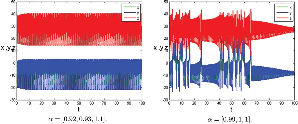
Figure 1: (Continued)

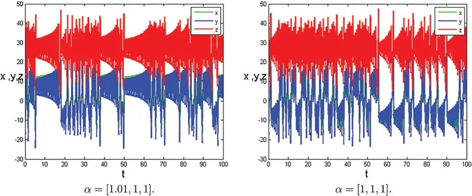
Figure 1:Time series plots of the systems(1)at[σ,ρ,β]=[10,28,8/3]with parameters α

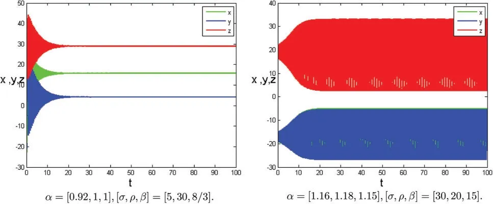
Figure 2: (Continued)

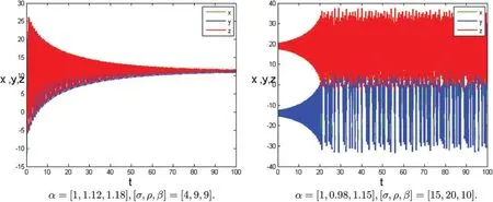
Figure 2:Time series plots of the systems(1)with different parameters

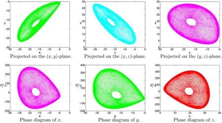
Figure 3:Numerical results for the systems(1)at α=[1.16,1.18,1.15],[σ,ρ,β]=[35,20,15],T=100

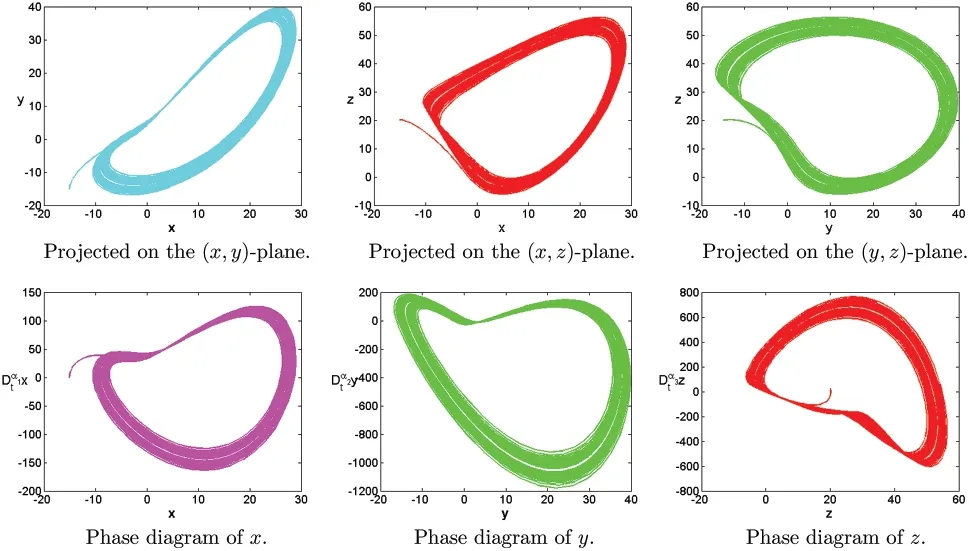
Figure 4:Numerical results for the systems(1)at α=[0.9,1.29,1.28],[σ,ρ,β]=[8,12,10],T=100

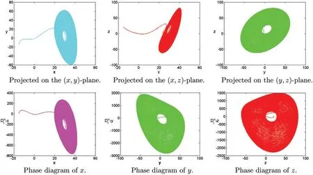
Figure 5:Numerical results for the systems(1)at α=[1.29,1.2,1.1],[σ,ρ,β]=[8,12,10],T=100

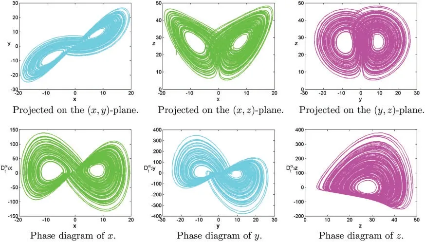
Figure 6:Numerical results for the systems(1)at α=[0.95,1.02,1.03],[σ,ρ,β]=[10,28,8/3],T=100

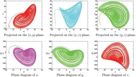
Figure 7:Numerical results for the systems(1)at α=[1.1,1.15,1.18],[σ,ρ,β]=[10,28,8/3],T=100

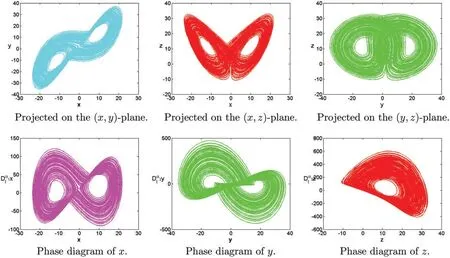
Figure 8:Numerical results for the systems(1)at α=[0.9,1.02,1.27],[σ,ρ,β]=[5,12,10],T=100

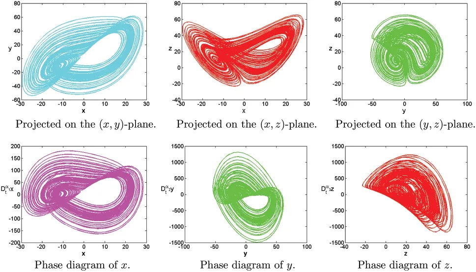
Figure 9:Numerical results for the systems(1)at α=[0.9,1.18,1.38],[σ,ρ,β]=[3,10,11],T=100

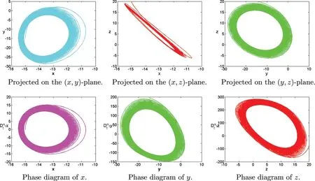
Figure 10:Numerical results for the systems(1)at α=[1,1.18,1.38],[σ,ρ,β]=[1,8,15],T=100

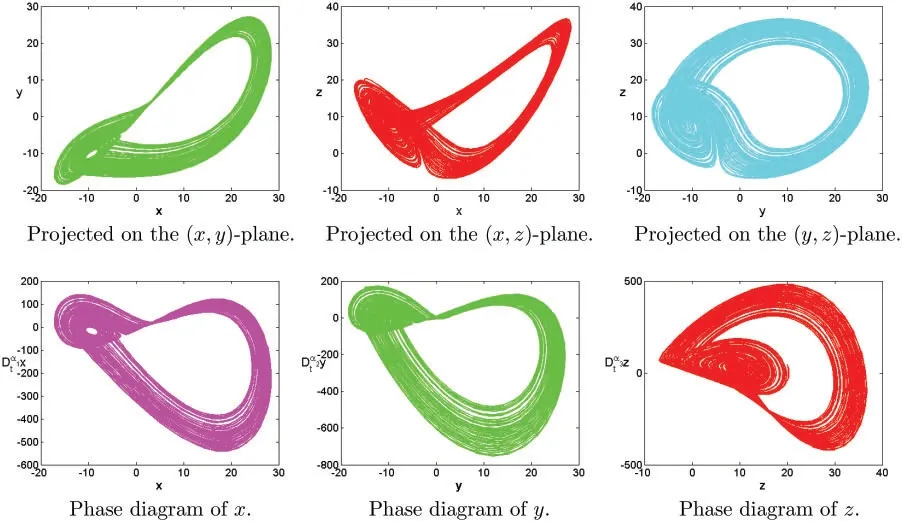
Figure 11:Numerical results for the systems(1)at α=[1.22,2.21,1.19],[σ,ρ,β]=[20,10,9]

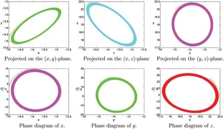
Figure 12:Numerical results for the systems(1)at α=[1,1.12,1.18],[σ,ρ,β]=[4,9,9],T=100

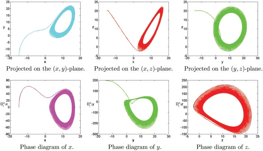
Figure 13:Numerical results for the systems(1)at α=[1,1.12,1.18],[σ,ρ,β]=[6,8,9],T=100

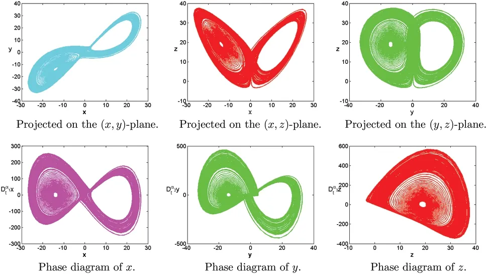
Figure 14:Numerical results for the systems(1)at α=[1,0.98,1.15],[σ,ρ,β]=[15,20,10],T=100

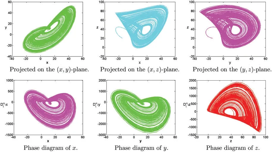
Figure 15: Numerical results for the systems (1) at α=[1.12,1.26,1.28],[σ,ρ,β]=[30,30,10],T=100

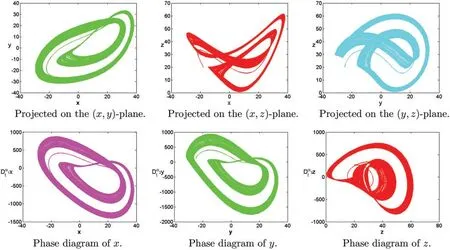
Figure 16: Numerical results for (1) at α=[1.35,1.25,1.2],[c1,c2,c3]=[−18,−25,20],[σ,ρ,β]=[35,15,9],T=100

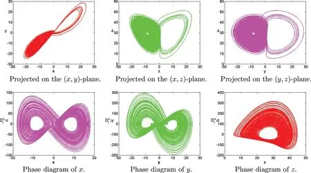
Figure 17: Numerical results for the systems (1) at α=[0.92,0.99,1.01],[σ,ρ,β]=[20,30,8/3],T=100

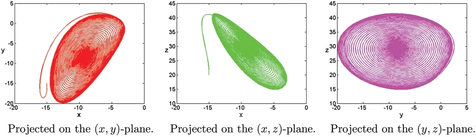
Figure 18:Numerical results for the systems(1)at α=[0.92,1,1],[σ,ρ,β]=[5,30,8/3],T=100

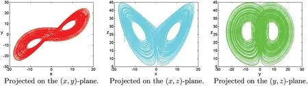
Figure 19:Numerical results for the systems(1)at α=[1,1,1],[σ,ρ,β]=[10,28,8/3],T=100

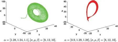
Figure 20: (Continued)

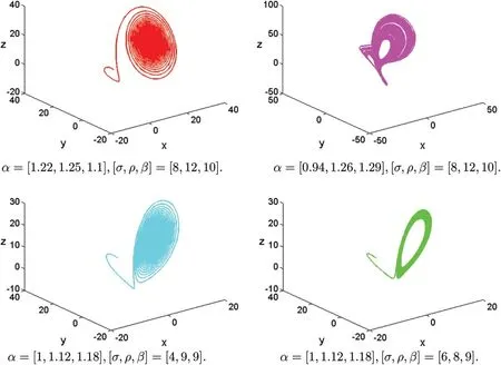
Figure 20:Chaotic attractor of fractional-order Lorenz systems(1)with different parameters

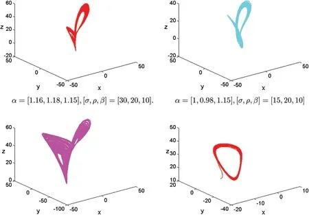
Figure 21: (Continued)

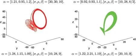
Figure 21:Chaotic attractor of fractional-order Lorenz systems(1)with different parameters

4 Conclusions and Remarks

In this paper,some complex dynamic behavior of fractional-order Lorenz chaotic systems are shown by using the present method.We observe many novel dynamic behaviors in numerical experiments which are unlike any that have been previously discovered in numerical experiments or theoretical studies.We investigate the influence ofα1,α2,α3on the numerical solution of fractionalorder Lorenz chaotic systems.The simulation results of integer order are in good agreement with those of other methods.The results presented in this paper suggested that the present numerical method is also readily applicable to a more chaotic system.

All computations are performed by the MatlabR2017b software.

Acknowledgement: The authors would like to express their thanks to the unknown referees for their careful reading and helpful comments.

Funding Statement: This paper is supported by the Natural Science Foundation of Inner Mongolia[2021MS01009]and Jining Normal University[JSJY2021040,Jsbsjj1704,jsky202145].

Conflicts of Interest:The authors declare that they have no conflicts of interest to report regarding the present study.