A Novel Localized Meshless Method for Solving Transient Heat Conduction Problems in Complicated Domains

Chengxin Zhang,Chao Wang,Shouhai Chenand Fajie Wang,＊

1College of Mechanical and Electrical Engineering,National Engineering Research Center for Intelligent Electrical Vehicle Power System,Qingdao University,Qingdao,266071,China

2Hisense(Shandong)Air Conditioner Co.,Ltd.,Qingdao,266100,China

ABSTRACT This paper first attempts to solve the transient heat conduction problem by combining the recently proposed local knot method(LKM)with the dual reciprocity method(DRM).Firstly,the temporal derivative is discretized by a finite difference scheme, and thus the governing equation of transient heat transfer is transformed into a non-homogeneous modified Helmholtz equation.Secondly, the solution of the non-homogeneous modified Helmholtz equation is decomposed into a particular solution and a homogeneous solution.And then,the DRM and LKM are used to solve the particular solution of the non-homogeneous equation and the homogeneous solution of the modified Helmholtz equation, respectively.The LKM is a recently proposed local radial basis function collocation method with the merits of being simple,accurate,and free of mesh and integration.Compared with the traditional domain-type and boundary-type schemes, the present coupling algorithm could be treated as a really good alternative for the analysis of transient heat conduction on high-dimensional and complicated domains.Numerical experiments,including two-and three-dimensional heat transfer models,demonstrated the effectiveness and accuracy of the new methodology.

KEYWORDS Local knot method;transient heat conduction;dual reciprocity method;meshless method

1 Introduction

Transient heat conduction exists widely in the thermal structure design of industrial equipment such as energy and chemical industry,as well as in the casting and heat treatment process of many new materials[1,2].Therefore,the study on transient heat conduction is very important for a long time.It is not easy work to find analytical solutions to practical engineering problems.Hence,the numerical simulation becomes an important way of approximating numerical solutions.

There are many kinds of conventional numerical methods applied to transient heat conduction problems, for instance, the finite element method (FEM) [3,4], the finite difference method (FDM)[5]and the boundary element method(BEM)[6,7].Among them,the FEM has been widely used in engineering and scientific calculation, and its mature commercial software has been widely used to analyze and simulate practical problems.There is no doubt that these traditional grid-type methods have their own advantages,but they still face many difficulties and challenges,such as complex mesh generation and other pre-processing processes,which affected the calculation accuracy and efficiency,especially for the complicated geometry.

In order to get rid of the complexity of mesh generation and reduce the time of preprocessing,various meshless methods have devoted considerable attention.These approaches include the elementfree Galerkin method [8-11], the reproducing kernel particle method [12-15], the meshless local Petrov-Galerkin method [16,17], the radial basis function collocation method (RBFCM) [18,19],the generalized finite difference method (GFDM) [20-23], the singular boundary method (SBM)[24,25],the method of fundamental solutions(MFS)[26,27]and the boundary knot method(BKM)[28,29],etc.The successful application of these meshless methods fully demonstrates their development prospect.However, each method is faced with more or fewer limitations while playing its own advantages.As the semi-analytical, strong-form, and boundary-type meshless collocation methods,they are difficult to apply to complex-geometry and large-scale problems due to their dense matrix characteristics.

For the above reasons,a new class of meshless collocation techniques,called the localized semianalytical meshless methods, has been proposed to solve various mathematical and mechanical problems.Such methods mainly include the localized method of fundamental solution(LMFS)[30],the localized singular boundary method(LSBM)[31],the localized Trefftz method(LTM)[32],and the localized boundary knot method (LBKM) [33].The LMFS and the LSBM use the singular fundamental solutions as the basis functions, the LTM employs the T-complete functions, and the LBKM uses the non-singular general solutions.The first two methods need to determine the fictitious boundary and the source intensity factor resulting from the source singularity, while the latter two methods can be used for numerical approximation directly.Recently, these schemes have been successfully applied to heat and mass transfer[34,35],acoustics[36],elastic mechanics[37,38],inverse problems[39,40]and other aspects.For details,see[41]and references therein.

Very recently,an improved LBKM called the local knot method(LKM)[42-44],is developed to solve the convection-diffusion-reaction and acoustic problems.The improved scheme is a local RBF method,and does not need the boundary of supporting subdomain and artificial nodes on it,which enhances the computational efficiency.Compared with other local semi-analytical meshless methods,this approach adopts the non-singular general solution instead of singular fundamental solution,and thus it avoids the evaluation of fictitious boundary and the original intensity factor.Furthermore,the heat transfer equation becomes a modified Helmholtz equation after time approximation,whose solution can be easily solved by using the LKM.Considering the simplicity, accuracy, efficiency,and large-scale simulation of the LKM, this study employed this approach to solve transient heat conduction problems.

Firstly,the temporal derivative is discretized by using the finite difference scheme.The governing equation is transformed into a non-homogeneous modified Helmholtz equation.Secondly,the solution of transformed equation is decomposed into a particular solution and a homogeneous solution of the corresponding homogeneous equation.Finally, the particular solution and the homogeneous solution are obtained by the dual reciprocity method(DRM)[28,45]and the LKM,respectively.The particular solution only satisfies the non-homogeneous equation, rather than boundary condition.However,the homogeneous solution satisfies both homogeneous equation and corresponding boundary conditions.It should be noted that that there are many ways to approximate a particular solution of non-homogeneous modified Helmholtz equation besides the DRM,such as the multiple reciprocity method,the polynomial approximation,and the radial basis function approximation.Among them,the DRM is a simple and popular technique addressing non-homogeneous terms and therefore is used in this study.

The outline of this article is as follows.Section 2 first briefly reviews the basic theory of the transient heat conduction problem, and then introduces the LKM and DRM.In Section 3, three numerical examples are presented to demonstrate the accuracy and validity of the proposed scheme.Finally,Section 4 provides some conclusions.

2 Mathematical Formulations

2.1 Governing Equation

A bounded domainΩwith boundaryΓ=∂Ωis considered.The governing equation of the transient heat conduction problems is indicated as

with initial and boundary conditions

whereddenotes the dimension of space,T(x,t) the temperature on the pointxat the timet,kthe thermal conductivity,ρthe mass density,cthe specific heat capacity,nthe outward unit normal vector,Qthe internal heat source,T0the initial temperature.(x,t)and(x,t)represent the known temperature and heat flux on the boundariesΓDandΓN,respectively.

2.2 Time-Advancing Scheme

The transient heat conduction problem is transformed into the modified Helmholtz equation by using the finite difference scheme to deal with the time variable.For the time span[tn,tn+1]⊂[0,t].The temperatureT(x,t)at any node in the object,its partial derivative with respect to time and the internal heat source can be approximated by

wherendenotes the time level,Δt=tn+1-tnis the time step.

Substituting Eqs.(5)-(7) into Eq.(1), the temperatureTn+1(x) at timetn+1can be obtained.The sorted formula is as follows:

It should be pointed out that the numerical solutionTn(x)in Eq.(8)can be obtained at timetn.

For convenience,Eq.(8)can be simplified as

in which

Noted that Eq.(9) is a non-homogeneous modified Helmholtz equation.Its solution can be decomposed into two parts(a particular solution and a homogeneous solution),namely,

The particular solution only satisfies the non-homogeneous equation,rather than boundary condition.However,the homogeneous solution satisfies both homogeneous equation and corresponding boundary conditions.The next two subsections will introduce the dual reciprocity method and the LKM for approximating particular solution and homogeneous solution,respectively.

2.3 Dual Reciprocity Method

Obviously, the particular solutionTp(x) should satisfy non-homogeneous equation Eq.(9),namely,

This study uses the dual reciprocity method to approximate the particular solutionTp(x).According to its basic idea,the right-hand term of Eq.(13)is expressed by[28]

Accordingly,the particular solutionTp(x)can be given by

whereψsatisfies

As we all know, there are many kinds of radial basis functions.The present study adopts the following function[28]:

Substituting Eq.(17)into Eq.(16),we can get the expression ofψ

2.4 Local Knot Method(LKM)

In this subsection, the LKM is used to approximate the homogeneous solutionTh(x).First, we give the corresponding governing equation and boundary conditions

In the LKM,N=ni+nb1+nb2nodes are discretized over the computational domainΩ,whereni,nb1andnb2are the numbers of interior nodes,Dirichlet boundary nodes and Neumann boundary nodes,respectively.Fig.1 shows the schematic diagram of the LKM.Considering an arbitrary node(here called the central nodex(0)) distributed in the computational domain, its m supporting nodesx(i),i= 1,2,...,mcan be easily determined.These nodes are contained in a circular or spherical subdomain called supporting domain.With regard to them+ 1 local nodes inside the supporting subdomainΩs,we can express the homogeneous solution as

or for brevity

whereI0is zero-order modified Bessel function of the first kind.

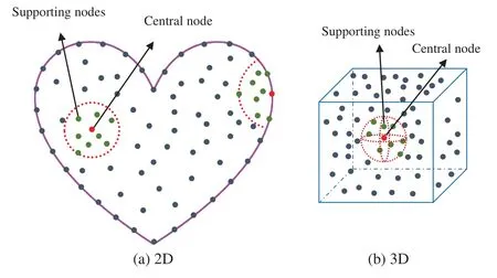
Figure 1:Schematic diagram of the LKM:(a)2D;(b)3D

Using the moving least squares theory,we define the following residual function:

whereω(i)denotes the weighting function.In our calculation,the spline weight function[16]is used

The unknown coefficientsς=(ς0,ς1,...,ςm)Tcan be obtained by minimizing the functionφ(T)with regard toς,namely,

Then,a matrix equation can be obtained,

where

Further,the vectorbin Eq.(29)can be recast as

In terms of Eqs.(28)-(30),ς=(ς0,ς1,...,ςm)Tcan be obtained by

Leti=0 and using Eq.(23),we have

In addition,the normal derivative can be calculated by

or for brevity

At internal nodes and boundary nodes,the following equations should be satisfied:

By combining Eqs.(36)-(38),we can obtain a linear system

whereEN×Nis a sparse coefficient matrix,Th= [T(1),T(2),...,T(N)]Tcontains the homogeneous solutions at all nodes,andhN×1is a vector consisting of right-hand term of and boundary data.After solving the above equation,the temperatureT(x)at all nodes can thereby be obtained by the following formula:

3 Numerical Results and Discussion

Three numerical examples are investigated to test the accuracy and effectiveness of the proposed scheme.To measure numerical accuracy,the following errors are adopted:

in whichWis the total number of test points,ukn(k= 1,2,...,W) anduke(k= 1,2,...,W) are numerical and exact solutions at the test point,respectively.It should be pointed out that the nodes in examples 1 and 2 are generated from MATLAB software and the nodes in example 3 are automatically generated from Hypermesh software.

3.1 Example 1:Rectangular Domain with a Hole

In the first example, we consider a transient heat transfer problem in a rectangular plate with a hole [46].The size parameters and boundary conditions of this model are given in Fig.2.The density, the specific heat and the heat conductivity areρ= 5000 kg/m3,c= 200 J/(kg · °C) andk=200 W/(m·°C),respectively.The initial temperature is taken to beT0=20°C,the temperature on the left boundary rises toT=500°C,while the right boundary maintains the initial temperature.Other boundaries are adiabatic.The temperatures at points A (0.07, 0.025) and B (0.075, 0.02) need to be studied and discussed in this example.Fig.3 shows the distribution of nodes in the computation.The interior of plate is discretized into 3853 nodes and its boundary is discretized into 200 outer boundary nodes and 31 inner boundary nodes.

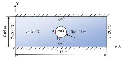
Figure 2:Dimensions and boundary conditions of the plate

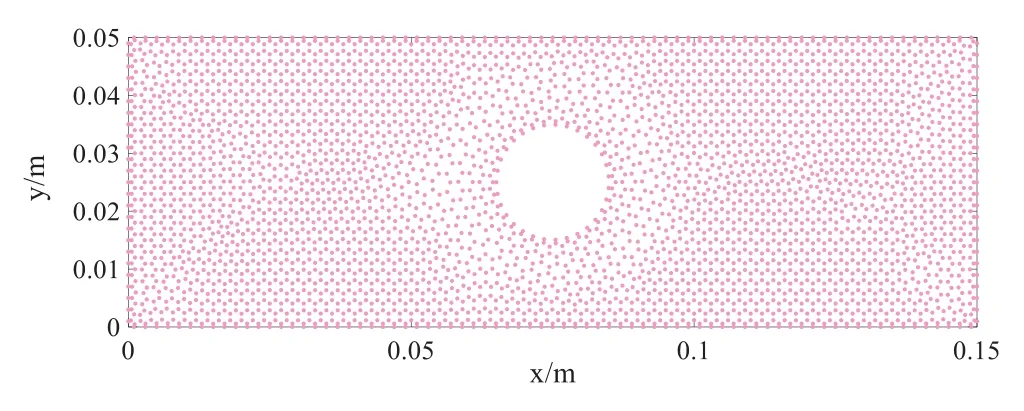
Figure 3:Nodal distribution of the LKM

In the calculation,we setm= 30 andΔt= 4 s.Since no analytical solution is available in this example,the finite element results calculated by COMSOL Multiphysics 5.4 are taken as the reference solution, in which the model is divided into 3853 domain elements.Fig.4 gives the comparisons of the calculated temperatures between the FEM and the LKM at the points A and B within 200 s.From Fig.4, it can be seen that the LKM results are in good agreement with those of the FEM, and the temperature at point A is higher than that at point B.In addition,when the time is less than 10 s,there is a certain deviation between the results of the LKM and the FEM,but with the increase of time,the deviation between them decreases and the temperature tends to be stable.

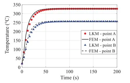
Figure 4:Temperature variation at points A and B with time

Then,we consider the numbers of supporting points asm= 20,30,40,50 to verify the accuracy and convergence of the LKM.Fig.5 shows the relative deviation curves of the FEM and the proposed method at point A.It can be clearly seen from Fig.5 that the deviations decrease rapidly at first,reach the optimal value and then tend to be stable as time goes on.When the number of supporting points is 20 and the time is 100 s,the minimum deviation is 1.148×10-6.At the 200 s,the deviations of the four cases are all less than 4.769×10-3,meeting the accuracy requirements.Furthermore,with the increase of supporting points,the relative deviations converge faster and reach the optimal value faster,indicating that LKM has good convergence.

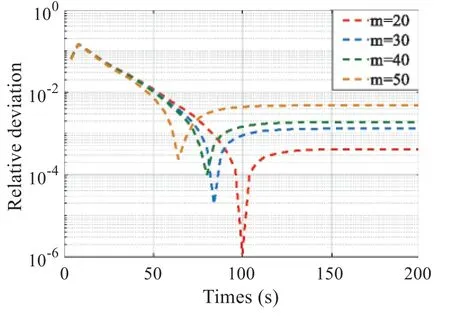
Figure 5:The relative deviation curves at point A

Figs.6-8 illustrate the temperature distributions calculated by the LKM and the FEM at 4,8 and 200 s, respectively.Obviously, the results near the hole have a little different at the beginning of the time period,but gradually become identical when the time goes to 200 s.

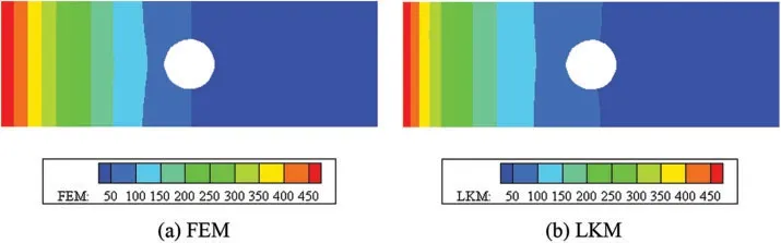
Figure 6:Profiles of temperature on the plate at time 4 s:(a)FEM;(b)LKM

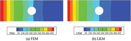
Figure 7:Profiles of temperature on the plate at time 8 s:(a)FEM;(b)LKM

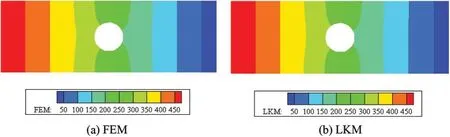
Figure 8:Profiles of temperature on the plate at time 200 s:(a)FEM;(b)LKM

3.2 Example 2:A Cube with Heat Generation

The LKM is applied to analyze the temperature field of the cubic domain in the second example.The shape parameters and initial temperature of the cube are shown in Fig.9a.Fig.9b shows the distribution of nodes in the computation, including 5832 boundary nodes and 1944 internal nodes.The thermal diffusivity is assumed to bea=k/ρc= 0.16 m2/s.The heat generation is expressed as[28]

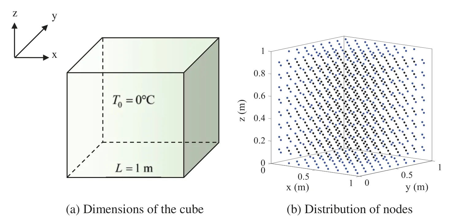
Figure 9:Dimensions and nodal distribution of the cube:(a)Dimensions of the cube;(b)Distribution of nodes

The analytical solution is given by

whereQ0/k=100°C/m2.

In this example, we consider two cases: (a) All the boundaries satisfy the Dirichlet boundary conditions;(b)The boundaryy=0 satisfies the Neumann boundary conditions,and the heat flux can be expressed aswhile the temperature is 0°C on the remaining boundaries.

In this example,the number of the supporting nodes is 60,and the time interval isΔt= 0.05 s.For the two different cases, Fig.10 shows the comparison of temperature on the line {(x,y,z)|0 ≤x≤1,y=z=0.5}at different times obtained by using the LKM and analytical expression.It can be plainly indicated that the developed method has good accuracy for the simulation of transient heat conductions with two kinds of boundary condition.In addition,it can also be noted that the error is slightly large whenx∈[0.4 0.6],but the error gradually decreases along with the time goes on.

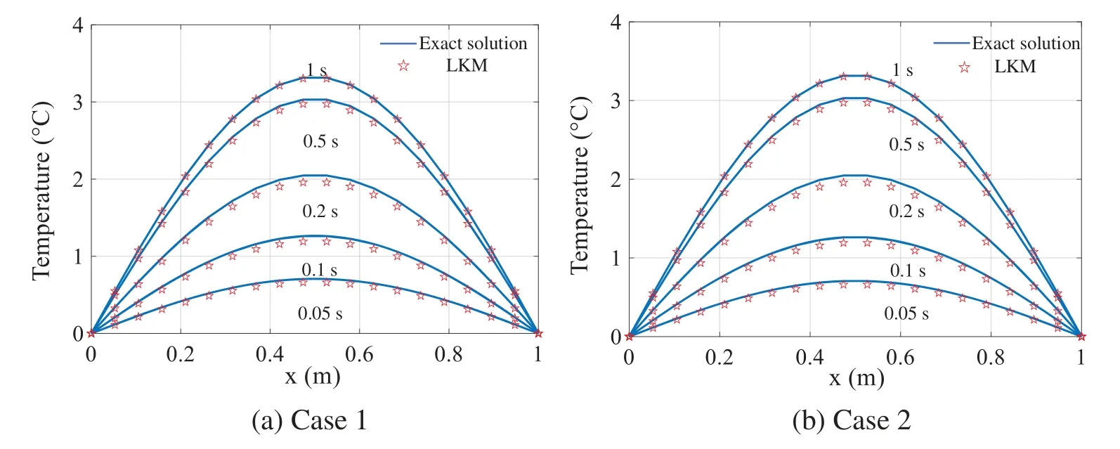
Figure 10: Temperature distributions on the line {(x,y,z)|0 ≤x ≤1,y = z = 0.5}: (a) Case 1;(b)Case 2

Additionally,Fig.11 plots the temperature curves with time marching for three internal points C(0.2,0.2,0.2),D(0.4,0.4,0.4)and E(0.6,0.6,0.6)for two cases and compares with the corresponding exact results.The results show that the method has high precision.

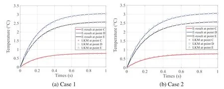
Figure 11:Distributions of temperature at different times at points C,D and E:(a)Case 1;(b)Case 2

By comparing the results of the LKM and the BKM in different cases, the accuracy and convergence of this method are carefully validated.With the increase of the total number of nodes,the variation of the errors and the condition numbers of the two methods are listed in Tables 1 and 2.As can be seen from Tables 1 and 2,although there are a few errors at some nodes,the results are still clear that the maximum and global errors of the two methods decrease with the increase of the number of nodes,and meet certain convergence trend.Next,we can conclude that when the total number of nodes is greater than 3211,the LKM is better than the BKM.Moreover,the LKM has fewer condition numbers regardless of the total number of nodes.In summary,the proposed LKM is high-precision,stable and convergent for solving 3D transient heat transfer problems.

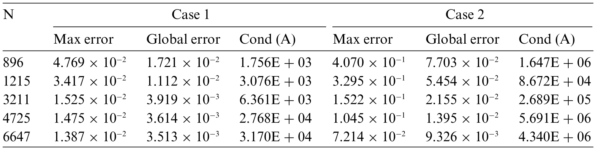
Table 1: Errors and condition numbers of the LKM under different cases

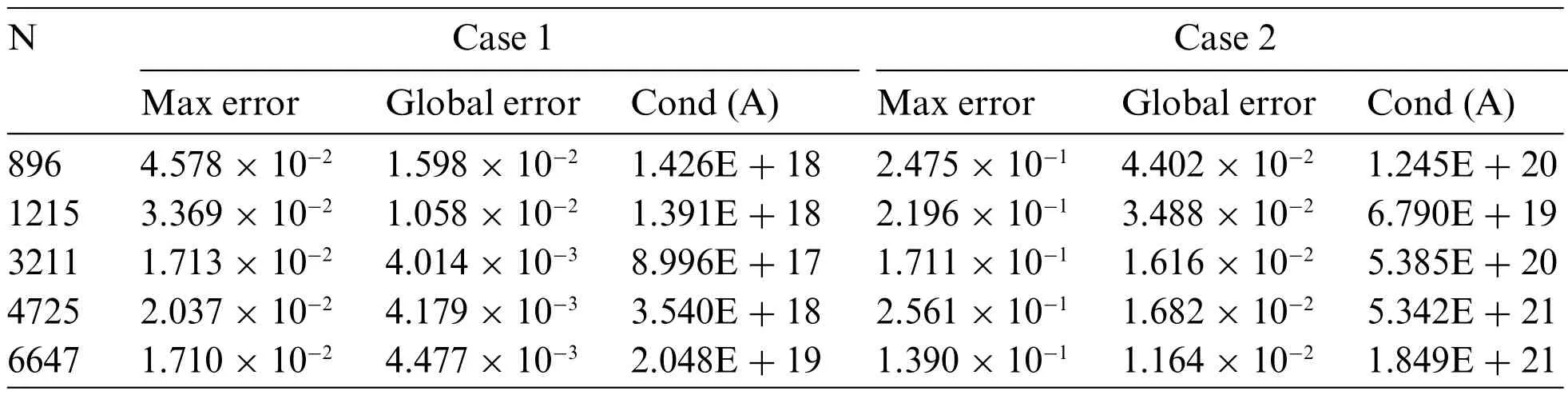
Table 2: Errors and condition numbers of the BKM under different cases

Finally,we can observe from Fig.12 that the distributions of absolute errors on the cross sectionz=0.5 in two cases are different.In case 1,it can be clearly seen that the absolute error in the center of the computational domain is largest(but less than 1.711×10-2),and gradually decreases from the center to the boundaries.In case 2,we can find that the absolute error on the boundaryy=0 is largest(but less than 7.21×10-2),and decreases sharply from it to other boundaries.The above phenomenon is mainly caused by different boundary conditions.

3.3 Example 3:A Hollow Cylinder

In order to verify the proposed LKM for simulating 3D transient heat conduction in a multiconnected domain, the third example considers is a hollow cylinder.Fig.13a plots the geometry parameters and boundary conditions of the model.The initial temperature is set to beT0= 500°C.The temperature at the top surface is suddenly decreased to 50°C,while the temperature stays the same at the bottom surface,and other surfaces are thermally insulated.The density,the heat conductivity and the specific heat areρ=7850 kg/m3,k=60 W/(m · °C)andc=460 J/(kg· °C),respectively.The discretization of nodes in the computation is shown in Fig.13b.There are 14146 nodes in the computation,of which 9706 are boundary nodes and the rest are internal nodes.Then,we continue to set FEM solution with more nodes(includes 229323 domain elements)than the proposed method as the reference solution.

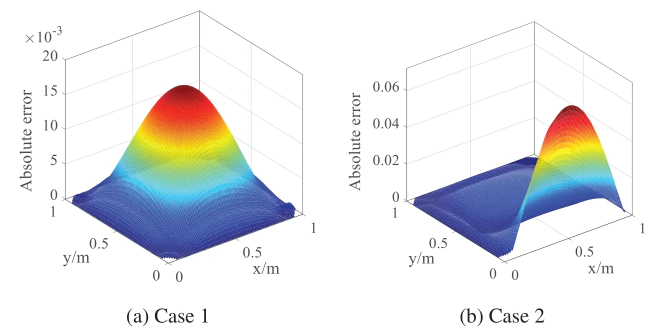
Figure 12:Distributions of absolute error on the cross section(z=0.5)for(a)Case 1;(b)Case 2

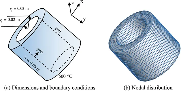
Figure 13: Dimensions, boundary conditions and nodal distribution of the hollow cylinder: (a)Dimensions and boundary conditions,(b)Nodal distribution

In this case,the number of supporting nodes is set to be 60.The length of each time step isΔt=1 s.Figs.14 and 15 depict the distribution of temperature field on the surface of the computational domain at the time 10 and 100 s.From Figs.14 and 15, it can be observed that the temperature increases gradually from top to bottom of the hollow cylinder.When the time advances to 100 s,the temperature changes in the calculation domain tends to be stable,and the results are almost identical for both the LKM and the FEM.We can carefully conclude that the LKM can also have high accuracy when using fewer nodes compared with the FEM.A large number of numerical experiments show that the proposed method has great potential in solving transient heat transfer problems,but the method needs to be further improved through continuous theoretical verification and engineering application.

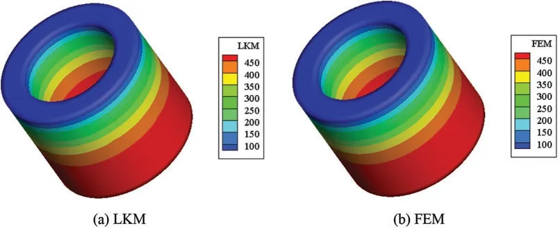
Figure 14:Contours of temperature at time 10 s:(a)LKM;(b)FEM

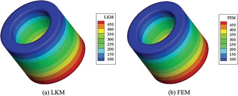
Figure 15:Contours of temperature at time 100 s:(a)LKM;(b)FEM

4 Conclusion

This paper presented a novel coupling algorithm of the LKM and the dual reciprocity method to simulate the transient heat transfer numerically.The LKM is a semi-analytical and local meshless method which uses the non-singular general solution as the basis function of interpolation.Unlike the existing conventional methods,the coupled approach avoids mesh division,reduces condition number and expands the simulation scale.

Numerical results of the three benchmark examples involving simply-connected and multiplyconnected domains have been investigated in detail.In the examples without exact solutions, our numerical results are compared with the FEM results from COMSOL software.Numerical experiments indicate that the proposed scheme is accurate and effective,and has small condition numbers.

This paper focuses on the application of the LKM in transient heat transfer problems,and shows its superior performance in solving such problems.However, there are still some issues that need to be addressed.The present study uses the Euler formula to discretize the time derivative, which has a certain impact on the accuracy and efficiency of the present method.Some more complex and accurate methods addressing the time derivative are interesting and will be discussed in more detail subsequently.Furthermore, the proposed methodology can be further optimized and improved to accurately solve the high-dimensional nonlinear heat transfer as well as the coupling heat transfer in complicated geometry.

Funding Statement:This work is supported by the National Natural Science Foundation of China(No.11802151),the Natural Science Foundation of Shandong Province of China(No.ZR2019BA008),and the China Postdoctoral Science Foundation(No.2019M652315).

Conflicts of Interest:The authors declare that they have no conflicts of interest to report regarding the present study.