RPNet: Rice plant counting after tillering stage based on plant attention and multiple supervision network

Xiodong Bi ,Susong Gu,Piho Liu ,Aiping Yng ,Zhe Ci ,Jinjun Wng ,Jinguo Yo

a School of Computer Science and Technology,Hainan University,Haikou 570228,Hainan,China

b Institute of Advanced Technology,Nanjing University of Posts and Telecommunications,Nanjing 210003,Jiangsu,China

c Agricultural Meteorological Center,Jiangxi Meteorological Bureau,Nanchang 330045,Jiangxi,China

Keywords: Rice Precision agriculture Plant counting Deep learning Attention mechanism

ABSTRACT Rice is a major food crop and is planted worldwide.Climatic deterioration,population growth,farmland shrinkage,and other factors have necessitated the application of cutting-edge technology to achieve accurate and efficient rice production.In this study,we mainly focus on the precise counting of rice plants in paddy field and design a novel deep learning network,RPNet,consisting of four modules:feature encoder,attention block,initial density map generator,and attention map generator.Additionally,we propose a novel loss function called RPloss.This loss function considers the magnitude relationship between different sub-loss functions and ensures the validity of the designed network.To verify the proposed method,we conducted experiments on our recently presented URC dataset,which is an unmanned aerial vehicle dataset that is quite challenged at counting rice plants.For experimental comparison,we chose some popular or recently proposed counting methods,namely MCNN,CSRNet,SANet,TasselNetV2,and FIDTM.In the experiment,the mean absolute error (MAE),root mean squared error (RMSE),relative MAE(rMAE)and relative RMSE(rRMSE)of the proposed RPNet were 8.3,11.2,1.2%and 1.6%,respectively,for the URC dataset.RPNet surpasses state-of-the-art methods in plant counting.To verify the universality of the proposed method,we conducted experiments on the well-know MTC and WED datasets.The final results on these datasets showed that our network achieved the best results compared with excellent previous approaches.The experiments showed that the proposed RPNet can be utilized to count rice plants in paddy fields and replace traditional methods.

1.Introduction

Rice is the second most important cereal crop in the world and accounts for 1/4 of the world’s total grain output with an annual output of approximately 800 Mt[1,2].Rice also has high economic value.For example,rice seeds can be utilized for starch production,and rice stalks can be used for feed and paper processing [3,4].However,owing to global warming,the cultivated farmland and water consumption for rice have decreased,resulting in a decline in production[5-7].Therefore,there is an urgent need to promote agricultural automation and precision agricultural technology to increase rice production.In China’s rice production,plant counts depend heavily on labor-intensive regional sampling and manual observations.Rice plant counting is a foundational task with numerous applications in rice production,including yield prediction,planting density selection,lodging resistance tests,disaster estimation,and rice breeding,etc.[8,9].Compared with the traditional manual count method,automatic plant counting saves human resources and has higher accuracy while avoiding direct contact between the observer and rice.

As the name implies,the purpose of plant counting is to accurately predict the number of plants against various complex backgrounds.In recent years,many crop counting methods have been reported.These can be roughly divided into three types counting methods: traditional machine learning (TML) methods,detection based deep learning (DDL) methods,and regression based deep learning (RDL) methods.

In TML methods,plant counting depends primarily on the TML algorithm.For example,Jin et al.[10] applied green pixel segmentation and PSO-SVM to estimate wheat plant density.Mojaddadi et al.[11] performed oil palm age estimation and counting from Worldview-3 satellite images and light detection and range(LiDAR) airborne imagery using an SVM algorithm.Through the extraction of spectral features from crop multispectral images and the application of MLR,Bikram et al.[12]estimated crop emergence.Although the above methods have achieved very good performance,all of these methods depend on manually selected image features according to specific crops or trees in their research.In DDL methods,crop counting is typically achieved using bounding box labeling and detection-based neural networks.The total number of bounding boxes in an output image is the number of predicted plants.For example,Hasan et al.[13] and Madec et al.[14] utilized a Fast RCNN architecture to realize wheat ear detection.A new multi-classifier cascade based method was proposed by Bai et al.[15] to realize rice spike detection and automatic determination of the heading stage.Yu et al.[16] studied the potential of the U-Net to provide an accurate segmentation of tassels from RGB images and then realized the dynamic monitoring of the maize tassel.However,these detection-based methods typically have drawbacks.First,the bounding box labeling is expensive and labor-intensive,especially for the high-throughput images collected by unmanned aerial vehicle (UAV).Second,because nonmaximum suppression is required to delete some candidate boxes,these models may ignore crowded and overlapping plants.Finally,time-consuming parameter tuning is typically required during the training stage [17].Compared to DDL counting methods,RDL methods have largely overcome the defects of DDL methods,do not require a tedious bounding box labeling,and perform better in dense scenes.Several achievements have been achieved in this regard.Rahnemoonfar and Sheppard [18] proposed a density regression model similar to that of the ResNet for counting tomatoes.Lu et al.[19] introduced a new maize tassel-counting model that included a novel upsampling operator to enhance visualization and counting accuracy.To realize citrus tree counting and locating,Osco et al.[20] considered individual bands and their combinations.A multicolumn convolutional network was presented by Lin et al.[21] to predict a density map and estimate the number of litchi flowers.Ao et al.[22] collected 5670 images of three types of rice seeds with different qualities and constructed a model to detect the thousand grain weight of rice.An active learning approach that automatically chooses the most relevant samples was proposed by Xiao et al.[23]to create an oil palm density map for Malaysia and Indonesia.Min et al.[24] proposed a maize ear phenotyping pipeline to estimate kernels per ear,rows per ear,and kernels per row in an interpretable manner.Although the above excellent RDL methods have been proposed,they still cannot be applied to accurately count rice plants in highthroughput UAV images.First,the crop objects selected by previous researchers were significantly different from rice plants in terms of shape,color,and appearance.Second,crop counting from the perspective of a drone has unique characteristics,such as long imaging distance,high-throughput imaging,and local texture loss.Third,we believe that a more effective feature fusion strategy and a more reasonable loss function can further improve network counting performance.

In this study,we propose a new rice plant counting network,RPNet,containing four modules: feature encoder,attention block,IDMG,and AMG.The proposed method first extracts shallow and deep features of the input image using the Feature Encoder.Next,because the extracted features are redundant,an attention block is adopted to highlight their unique information and realize a more effective feature fusion.Finally,the IDMG and AMG modules are presented to maintain accurate counting functions and regress the output density map.Moreover,we propose a new loss function(RPloss) that fully considers different sub-loss functions that supervise the training process of our network to realize rice plant counting.For experimental comparison,we selected classic networks such as MCNN and CSRNet and recently proposed competitive networks such as FIDTM and TasselNetV3.The source code for the RPNet is available at https://github.com/xdbai-source/RPNet.

2.Materials and methods

In this section,we will provide a detailed introduction to the network pipeline of the RPNet we have designed.Additionally,we will introduce the datasets URC [25],MTC [26] and WED [14]used in our experiments.

2.1.Framework overview

The main structure of our proposed network is illustrated in Fig.1.For the input imageI,feature encoder module was first utilized to extract its featuresF∈RC×H×W,whereC,HandWrepresent the number of channels,height,and width,respectively.Second,the featuresf1-f4extracted from the feature encoder were sent to the attention block to highlight the difference between the shallow and deep features and preserve the effective features.In the IDMG module,F4was employed to perform layer-by-layer upsampling for feature fusion,and obtain the initial density map (IDM)for rice counting.Using the same method,the attention map(AM)was generated for background suppression in the AMG module.The above IDM and AM were then multiplied to obtain the final output density map.In Fig.1A,the dot map is a 0-1 matrix indicating the labeled plant positions of an input image.The density map was obtained via the convolution of the above dot map.As shown in Fig.1A,ground-truth density map was obtained by down-sampling the density map and then used to supervise the network predicted density map.Next,ground-truth AM was applied to supervise the AM generated by the AMG obtained using the method described in section 2.4.

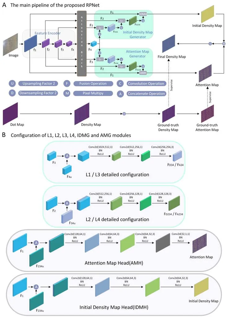
Fig.1.The network structure of the proposed RPNet.

2.2.Attention block

In Feature Encoder,VGG16 [27] was adopted to obtain shallow and deep features fromf1tof4.Considering the excellent spatial/channel feature extraction and fusion ability of the CBAM [28],it was first introduced into rice plant counting research and applied as the main part of the attention block to enhance the differences between features and enable feature fusion.Fig.2 shows the structure of the CBAM.The channel-dimension attention weightsMCwere first calculated using channel attention module.These weights were then multiplied with the input featurefto obtain the channel-refined featuref’.Next,using the spatial attention module,the spatial dimension attention weightsMSwere obtained.Finally,MSwas multiplied by the channel-refined featuref’to generate the refined featureF.The detailed structures of the channel attention module and spatial attention module are presented below.

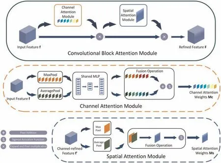
Fig.2.Architecture of the CBAM.

As shown in Fig.2,in the channel attention module,the input featuref∈RC×H×Wwas first utilized via average pooling and global maximum pooling along theH×Wdimension to obtain featuresfCAvg,fCMax∈RC×1×1respectively.Then,fCAvgandfCMaxwere integrated through the shared fully connected layer respectively.Next,after the element-wise summation offCAvgandfCMax,the channel attention weightsMCwere calculated by the sigmoid activation function.In the spatial attention module,the input channel-refined featuref’was first subjected to average pooling and maximum pooling along the channel dimension respectively to obtain featuresfSAvg,fSMax∈R1×H×W.After that,fSAvgandfSMaxwere fused through a convolution layer.Finally,we obtained the spatial attention weightsMCthrough the sigmoid activation function.

2.3.IDMG and AMG modules

As shown in Fig.1A,the IDMG module comprisesL1,L2,an upsampling operation and initial density map head(IDMH).Adopting a similar structure,the AMG module was composed ofL3,L4,an upsampling operation,and an attention map head (AMH).More detailed configuration information regarding the IDMG and AMG is provided in Fig.1B.In the IDMG module,F4was upsampled twice and then sent toL1withF3to obtainFD34.In this process,L1realizes information fusion of different scales and depths by stacking the convolution layers.Similarly,FD34was upsampling twice,and merged byL2withF2to achieveFD234,whereL2integrates information from different scales and depths fromF2andFD34.Finally,we upsampleFD234twice,and fused it withF1in the IDMH to generate the IDM.The size of the IDM was 1/2 that of the original input image.Through the aforementioned continuous fusion operations,our model can capture information from multiple scales and depths to suppress the scale transformation of the samples.

To reduce the effect of noise on the image background,we designed an AMG module for the proposed RPNet.In the AMG module,F4was first upsampled twice and then merged withF3usingL3to obtain the fused attention featureFA34.Next,FA34was upsampled twice,and merged withF2to obtainFA234,whereFA234integrated the attention information fromF2andFA34.Finally,we upsampledFA234twice,and fused withF1in the AMH to generate the AM.Its size was also 1/2 of the original input image.By fusing the attention information at different scales and depths,the model accurately focused on the feature regions of interest in scenes with large-scale changes.

After obtaining the IDM and AM,the final density map (FDM)was calculated using Eq.(1),where conv represents the convolution operation,and ‘⊙’ is an element-wise multiple.

2.4.Multiple supervision loss function

In this section,we introduce the generation process of the ground-truth density mapDgtand the ground-truth AMAgt.Subsequently,we introduce the newly proposed multiple supervision loss function,RPloss.

If δ ·（）is defined as an impulse function,it can applyto represent a plant at image positionxi.We then employed Eq.(2)to describe the dot map withNplants,namelyH（x）.Finally,similar to the method used by [29],we convolved H（x）with the fixed Gaussian kernelGσ（x）to obtain the ground-truth density map given in Eq.(3).

The ground-truth density map generated using Eq.(3) can be regarded as a probability map of plant appearance.Therefore,for image pixels with zero value,we consider that they do not contain plants and regard them as background.Conversely,for pixels with nonzero values,we assume that they may contain plants and regard them as foreground.Based on the above considerations,we regard the foreground areas as the ground-truth AMAgtand expect our model to pay more attention to these areas.Consequently,Eq.(4) can be applied to obtain the ground-truth AM.

In the following,we describe the proposed multiple supervision loss function,RPloss.During the network training process,the above obtained ground-truth density map and ground-truth AM were utilized for network supervision and learning.

For AM supervision,we chose the binary cross-entropy lossLbceas our sub-loss function as shown in Eq.(5),whereKrepresents the batch size,andrepresent theithground-truth AM and the predicted AM,respectively.

For the density map supervision,we chose L1loss to supervise the counting performance and further used L2loss to improve the quality of the generated density map.L1loss and L2loss can be written as Eqs.(6)and(7),respectively,whereandrepresent the ground-truth density map and the predicted density map,respectively.

Moreover,we introduced a probabilitypvalue representing the correct manual labeling.The probability of incorrect labelling was1-p.Next,we recorded the area in the input image that contained a plant as a positive domain and that containing no plant as a negative domain.Consequently,if a pixelxmin the ground-truth density map was greater than zero,the probability falling in the positive domain isp,and the probability falling in the negative domain is 1-p.If the pixel value was less than or equal to zero,it was regarded as a background point.Because background points require no labeling,we assumed thatxmwas error free;therefore,the probability of labeling it in the positive domain is 0,and the probability of labeling it in the negative domain is 1.Thus,equations (8) and (9) can be used to express the above operation.

We calculated the number of predicted density maps in the positive and negative domains using Eqs.(10) and (11):

We hope that the sum of the positive domainCpostended toward the ground-truth countCgt,and the sum of the negative domainCnegtended toward zero to suppress the background.Hence,our positive-negative lossLPNcan be expressed as:

To sum up,our multiple supervision loss function was:

where λ1,λ2and λ3are hyperparameters.

In the experiment,the magnitude of each sub-loss function of Eq.(13) was quite different.Therefore,for better compatibility and adaptation between sub-loss functions,we set their weights λ1,λ2,λ3into 1,10-3and 10-4,respectively.In our UAV-based rice plant counting dataset,plants were approximately evenly distributed,and there were relatively few scenes with plant occlusion.After completing the manual labeling of the URC dataset,a twowheeled manual review was conducted.Therefore,the manual labeling errors were negligible,and we setPinLPNto 1 in this case.

2.5.Datasets

In this study,we focus on the accurate rice plant counting in paddy fields based on high-throughput images collected by an UAV.The proposed RPNet was evaluated using our recently proposed UAV-based rice counting dataset URC.To further verify the counting capability of the proposed network,the MTC and WED datasets were introduced in our experiment.Below,we introduce each dataset separately.

URC: This dataset is our recently proposed dataset containing 355 high-resolution(5472×3468)RGB rice images collected using low-altitude drone (DJI Phantom 4 Advanced) and 257,793 manually annotated points.During the manual labeling of the URC dataset,we followed the labeling method described by Xiong et al.[30]and placed a dot annotation at the center of each rice plant.We wrote a script using MATLAB R2018 to improve the efficiency of the manual labeling and facilitate the display of the labeled annotations.In the URC,246 images were randomly selected for training,and the remaining 109 images were used for testing.Each image contains 84-1125 rice plants,with an average of 726 plants per image.The dataset was challenged by various light conditions.The images were taken at a height of 7 m using DJI GS Pro in Nanchang (28°31′10′′N,116°4′6′′E),Jiangxi,China.Each pixel in the URC dataset images corresponds to approximately 0.01 square centimeters.All collected images were stored in the JPG format.

MTC: It is the well-known maize tassel counting dataset containing 361 high-resolution RGB maize images with three types of image resolutions: 3648 × 2736,4272 × 2848 and 3456 × 2304.In the dataset,186 images were used for training,and 175 images were used for testing.All images were automatically collected using a camera(E450 Olympus)fixed in four fields:Zhengzhou (34°16′N,112°42′E),Henan,China;Tai’an (39°38′N,116°20′E),Shandong,China;Gucheng (30°53′N,111°7′E),Hubei,China;Jalaid (46°52′N,122°32′E),Inner Mongolia,China.The shooting height was 5 m,except in Gucheng,which was 4 m.Each maize tassel in the dataset was manually labeled using a bounding box.These bounding-box annotations were directly transformed into dot annotation by calculating their central coordinates.

WED: It is a well-known wheat ear detection dataset used to count wheat ears.It contains 236 high-resolution RGB images of six different types of wheat ears,with an image resolution of 6000 × 4000.In the dataset,165 images were used for training,and 71 images were used for testing.Each image contains 80-170 wheat ears.The entire dataset contained 30,729 wheat-ear images.Those images were captured by SONY ILCE 6000 in Gréoux les Bains,France (43.7°N,5.8°E),at a height of 2.9 m.Each wheat ear was manually labeled with a bounding box by‘LABELIMG’[14].

Representative images from the three datasets are shown in Fig.3.Images were selected from the URC,MTC,and WED datasets from the top to bottom rows.

Fig.3.Some representative images in the URC,MTC and WED datasets.The images in rows 1 to 3 are from the URC,MTC,and WED datasets,respectively.

3.Results

3.1.Implement details

VGG16_bn with parameters pre-trained on ImageNet,was employed as the backbone of the feature encoder.The number of training epochs was set to 500.The batch size was 3,and the initial learning rate,Lr,was set to 10-4.For the three datasets,we first resize all original images and then randomly cropped,flipped,and scaled each training image for image augmentation.The Adam algorithm with a step factor of 10-5was used as the optimizer.In the spatial attention module in CBAM,we set the convolution kernel of the convolution layer in fusion operation to,whereHiis the height of the input feature map.The resizing sizes or downsampling ratios for different datasets,crop sizes,and the σ size used for the ground-truth density map generation are all listed in Table 1.All experiments were based on the Pytorch framework and accelerated using an RTX 3090.

Table 1Image preprocessing settings of each dataset.

3.2.Evaluation metric

To evaluate the counting performance of the different approaches,we adopted the MAE,RMSE,rMAE and rRMSE as evaluation metrics.The above four indicators can be expressed as equations (14) to (17):

whereNis the number of images,andziandare ground-truth count number and predicted count numbers of theithimage,respectively.

3.3.Comparison with state-of-the-art methods

To evaluate the proposed RPNet rice plant counting method,it was compared with state-of-the-art counting approaches using the URC rice plant dataset.In order to evaluate the proposed RPNet method,it was compared with some classic counting methods(MCNN,CSRNet and SANet)and recent proposed counting methods(TasselNetV2 and FIDTM)on the URC dataset.To test the feasibility of the RPNet for other crop counting tasks,the MTC and WED datasets were applied in our experiment.In the following section,we introduce comparison experiments on these three datasets.

The performance of the different counting methods on the URC dataset are listed in Table 2.The MAE and RMSE of our RPNet obtained the lowest values 8.3 and 11.2 on this dataset,respectively.An improvement of 17.8% and 16.4% compared to the second-best SANet in the experiment.The rMAE and rRMSE values of the proposed network were 1.2% and 1.6%,respectively.Table 2 indicates the accuracy and robustness of our network.To further demonstrate the counting performance of our network,Fig.S1 shows some final output density maps for the URC dataset.

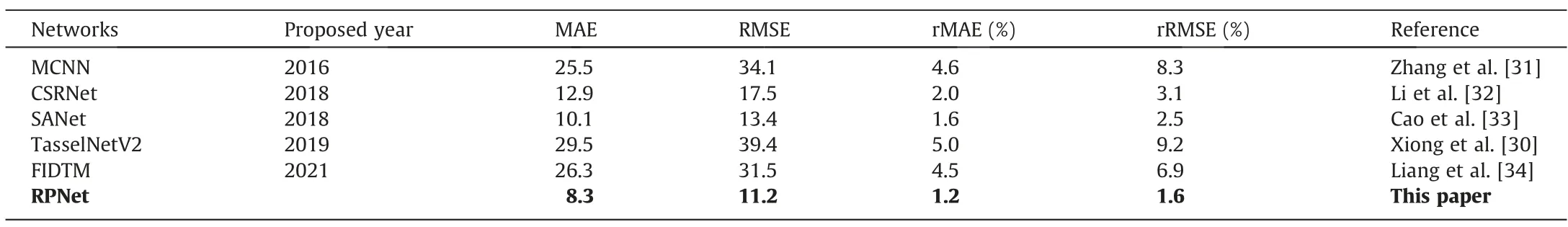
Table 2The performance of different methods on the test set of the URC dataset.

In Fig.S1,the five columns from left to right show the input test images,the ground-truth density maps,and predicted density maps generated by the RPNet,SANet and CSRNet respectively.‘GT’ and ‘PD’ denote the manual ground-truth and the network predicted count values,respectively.As shown in Fig.S1,the generated density map indicates that our model accurately counted rice plants.Furthermore,the network estimated density maps were similar to the ground-truth density maps.This indicates that the network estimated density map was of very high quality.As shown in the first and second rows of Fig.S1,to a certain extent,RPNet can deal with the scene of sunlight reflection in rice fields.Even in the case of strong sun reflection,the density map estimated using RPNet was essentially the same as the ground-truth density map.It’s interesting that SANet also shows a good ability to resist light reflection.However,as shown in the second,third,and fourth rows of Fig.S1,the density maps predicted by RPNet were better than those predicted by SANet.Moreover,the density maps generated by CSRNet were similar to the ground-truth density maps.However,the counting results were not as accurate as those of the proposed RPNet.We believe that the good counting accuracy of RPNet was owing to the effective integration of the four modules and the ability of RPloss to achieve effective supervision learning during the training stage.In future research,sun-glint suppression can also be achieved by improving the imaging method and implementing it in image preprocessing[35].To address this issue,researchers can acquire UAV images using both RGB and near-infrared cameras and use the near-infrared images to correct for the sun-glint effect in the RGB images.

For the MTC dataset,the MAE and RMSE of the proposed method also achieved the best results of 3.1 and 5.0,respectively,as listed in Table 3.Compared to the second-best SFC2Net,the MAE and RMSE improved by 38% and 46%,respectively.The rMAE and rRMSE of RPNet were 20.0% and 46.1%,respectively.RPNet provided rMAE and rRMSE results comparable to those of these methods.Fig.S2 shows the final output density maps for the MTC dataset.As shown in the first and second rows of Fig.S2,the RPNet performed well in both dense and sparse scenes.In the third row of Fig.S2,the newly sprouted maize tassels looked very similar to the surrounding leaves owing to changes in illumination.In this chaotic background scenario,our RPNet still distinguished the maize tassels from the background.We believe that the good performance of the RPNet was derived from the introduction of the plant attention block module and effective background suppression strategies that allowed the network to adapt to changes in light intensity and more effectively focus on the maize tassels in the image.As shown in the second and third rows of Fig.S2,the density maps generated by the SANet and CSRNet were unclear owing to interference from the image background.Compared with the SANet and CSRNet,the RPNet had a better counting accuracy and higher-quality predicted density map.We believe that this was mainly because RPNet was better at suppressing the image background.

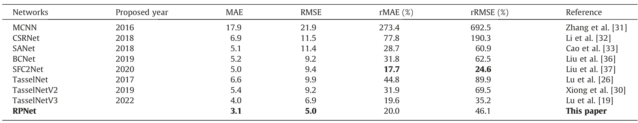
Table 3Performance of different methods on the test set of the MTC dataset.

The counting performances of different methods on the WED dataset are listed in Table 4.The proposed RPNet obtained the best MAE and RMSE,which were 4.0 and 4.9,as show in Table 4.Although the improvement was not significant compared with the second-best method,it was very competitive because the images all showed the characteristics of a messy background and dense wheat ear distribution.In Fig.S3,the five pictures differ in terms of image background and light intensity and without the contrast of the ground-truth density map,it is difficult for the human eye to identify all wheat ears.The estimated density map in the third column of Fig.S3 shows that RPNet accurately identified plants and achieved a counting performance.Simultaneously,we observed less background noise.As shown in the third and fifth rows of Fig.S3,the density maps generated by the SANet and CSRNet were not similar to ours.The results obtained by the RPNet indicate that the AM generated in the proposed RPNet was welltrained with the help of the presented RPloss.Thus,the RPNet effectively distinguished wheat ears from complex image backgrounds.

3.4.Ablation experiments

In this portion,we introduce the ablation experiments to demonstrate the effective configuration of the presented network.All the ablation experiments were conducted on the URC dataset.In the first ablation experiment,we demonstrate the impact of the hyper-parameter σ in the experiment.The value of σ represents the size of the fixed Gaussian kernel which is used to generate the ground-truth density map.The experimental results regarding this hyper-parameter in Table S1 show that our network performed best when σ was set to 6.When σ was small,some detailed plant features were lost because the window of the fixed Gaussian kernel could not completely cover the plant region.When σ was too large,the window of the fixed Gaussian kernel was beyond the plant region,and some interference information was included in the generated ground-truth density map and slightly reduced the counting performance of the network.

We performed another ablation experiment to demonstrate the effectiveness of each sub-loss function.All the related results are given in Table S2,and ‘√’ indicates that we utilized this sub-loss function.As shown in Table S2,the best performance of our network was obtained when all the sub-loss functions were employed.This experiment verified the effectiveness of the multiple supervision loss functions we designed in the proposed RPNet.By comparing the second row with the sixth row and the fifth row with the eighth row of Table S2,we find that the proposed LPNimproved the counting performance.By comparing the sixth line with the eighth line,we found that the AM effectively suppressed the background and improved the counting accuracy.

Additionally,we performed an ablation experiment to analyze the weight hyperparameters λ1,λ2and λ3in the RPloss.The comparative experiments were based on the URC dataset.The results of the different hyperparameters are listed in Table S3,where rows 1-6 represent the ablation experiments for λ1.In these sixexperiments,we fixed the parameters λ2and λ3,then utilized different parameters λ1to compare the counting performance of the proposed RPNet on the URC dataset.Similarly,rows 7-12 represent the ablation experiments for λ2.Rows 13-18 are the experiment results for λ3.In the initial experiments,we found that the magnitude of each sub-loss function was significantly different.We believe that the weight hyperparameters were not only related to the importance of different sub-loss functions,but also to the magnitudes of those loss values.Therefore,for better compatibility and adaptation between the sub-loss functions,we set the weights λ1,λ2and λ3to 1,10-3and 10-4,respectively,to balance the different sub-loss values.As shown in Table S3,the weights we chose were good.In fact,it was difficult to determine optimal hyperparameters and we proposed a feasible option for these weight hyperparameters.Researchers can utilize other methods to obtain better weights and further improve network performance.In future research,the selection of neural network hyperparameters may be a promising direction.

Finally,we analyzed the running efficiency of the proposed RPNet on a GPU server equipped with an RTX 3090.Table S4 lists the running efficiency of the different networks.As shown,the FPS of the neural network was closely related to the number of parameters and FLOPs.The running efficiency of the RPNet reached 3.57HZ FPS and was comparable with that of the SANet.Although there were fewer network parameters in the SANet,its running time was relatively long,mainly because the SANet adopts a series of transposed convolutions.In this study,frequent rice counting was unnecessary.Therefore,we did not need a rice counting network with high running efficiency.

4.Conclusions

In this study,we proposed a powerful rice plant counting network (RPNet) that accurately counts the number of rice plants in a paddy field based on a UAV vision platform.The main contributions of this study are as follows: Firstly,the presented RPNet can accurately count the number of rice plants in paddy field based on a UAV vision platform.In the experiment,the RPNet was evaluated using our recently proposed rice plant dataset,URC.Its performance surpassed that of many state-of-the-art methods for rice plant counting tasks.Additionally,the MTC and WED datasets were used in our experiment.Our network achieved the best performance for both datasets.This demonstrates that our network has the potential for other plant-counting tasks.Our network has an accurate rice plant counting ability and is highly competitive compared with other excellent counting approaches.Secondly,we propose an efficient loss function called RPloss.This loss function considers different sub-loss functions that achieve multiple supervision during network training and ensures the validity of network parameter learning.Lastly,the convolutional block attention module(CBAM)attention module is introduced into rice plant counting.It was applied as a rice plant Attention Block in the RPNet pipeline to extract and fuse multi-scale feature maps.In conclusion,experiments showed that the proposed network can be employed for the accurate counting of rice plants in paddy field,thereby replacing the traditional tedious manual counting method.

CRediT authorship contribution statement

Xiaodong Bai:Conceptualization,Methodology,Funding Acquisition,Writing-Review,Project Administration.Susong Gu:Methodology,Software,Validation,Writing.Pichao Liu:Conceptualization,Methodology.Aiping Yang:Resources,Formal Analysis,Investigation.Zhe Cai:Formal Analysis,Investigation.Jianjun Wang:Resources,Formal Analysis.Jianguo Yao:Project Administration,Funding Acquisition.

Declaration of competing interest

The authors declare that they have no known competing financial interests or personal relationships that could have appeared to influence the work reported in this paper.

Acknowledgments

The authors would like to thank the field management staff at the Nanchang Key Laboratory of Agrometeorology for their continued support of our research.Authors also would like to thank Shiqi Chen,Tingting Xie,Xiaodi Zhou,Dongjun Chen and Haocheng Li for their contribution to manual image labeling.Thanks Shiqi Chen and Tingting Xie for contributing to the language revision.This work was supported by the National Natural Science Foundation of China (61701260 and 62271266),the Postgraduate Research &Practice Innovation Program of Jiangsu Province (SJCX21_0255),and the Postdoctoral Research Program of Jiangsu Province(2019K287).

Appendix A.Supplementary data

Supplementary data for this article can be found online at https://doi.org/10.1016/j.cj.2023.04.005.