
Pollutant mixing and transport process via diverse transverse release positions in a multi-anabranch river with three braid bars
2013-06-22 13:25ZulinHUAWeiJINingningSHANWeiWU
Water Science and Engineering 2013年3期
Zu-lin HUA*, Wei JI, Ning-ning SHAN, Wei WU
1. Key Laboratory of Integrated Regulation and Resource Development on Shallow Lakes, Ministry of Education, Hohai University, Nanjing 210098, P. R. China
2. College of Environment, Hohai University, Nanjing 210098, P. R. China
3. National Engineering Research Center of Water Resources Efficient Utilization and Engineering Safety, Hohai University, Nanjing 210098, P. R. China
Pollutant mixing and transport process via diverse transverse release positions in a multi-anabranch river with three braid bars
Zu-lin HUA*1,2,3, Wei JI1,2,3, Ning-ning SHAN1,2,3, Wei WU1,2,3
1. Key Laboratory of Integrated Regulation and Resource Development on Shallow Lakes, Ministry of Education, Hohai University, Nanjing 210098, P. R. China
2. College of Environment, Hohai University, Nanjing 210098, P. R. China
3. National Engineering Research Center of Water Resources Efficient Utilization and Engineering Safety, Hohai University, Nanjing 210098, P. R. China
A multi-anabranch river with three braid bars is a typical river pattern in nature, but no studies have been conducted to describe mixing characteristics of pollutants in the river. In this study, a physical model of a typical multi-anabranch river with three braid bars was established to explore the pollutant mixing characteristics in different branches. The multi-anabranch reach was separated into seven branches, B1, B2, B3, B4, B5, B6, and B7, by three braid bars. Five tracer release positions located 2.9 m upstream from the inlet section of the multi-anabranch reach were adopted, and the distances from the five positions to the left bank of the upstream main channel were 1/6B, 1/3B, 1/2B, 2/3B, and 5/6B(Bis the width of the upstream main channel), respectively. The longitudinal velocities and pollutant concentrations in the seven branches were measured. The planar flow field and mixing characteristics of pollutants from the bottom to the surface in the multi-anabranch river were obtained and analyzed. The results show that the pollutant release positions are the main influencing factors in the pollutant transport process, and the diversion points and pollutant release positions jointly influence the percentage ratios of the pollutant fluxes in branches B1, B2, and B3 to the pollutant flux in the upstream main channel.
multi-anabranch river; braid bar; pollutant mixing characteristic; pollutant transport process
1 Introduction
In nature, there are several typical river patterns, such as a straight river, a meandering river, a braided river with one bar, a multi-anabranch river with several bars, etc. A great deal of research has been focused on the process of pollutant transport in straight rivers andmeandering rivers (Chau 2000; Deng et al. 2001; Zeng et al. 2008; Guymer 1998; Baek et al. 2006; Boxall and Guymer 2007; Seo et al. 2008).
At present, there have been a certain amount of studies on braided rivers with one bar. They mainly focus on the flow characteristics, sediment transport, and riverbed evolution of braided rivers. Flow in curved channels with a point bar was studied by Dietrich and Smith (1983). The results showed that a secondary circulation composed of outward flow at the surface and inward flow near the bottom extended across the entire width in a channel with bed topography that did not vary in the downstream direction. Holly and Yang (1985) presented a computational method and its application to a northern braided river. In the method, the flow energy equation, sediment continuity equation, bed armoring process, and bed material sorting process were computed separately but iteratively within a computational time step. The distributions of discharges and current velocities in braided channels of a flatland river under natural conditions and with the implementation of various engineering measures were obtained by Salikov (1989). Richardson and Thorne (1998) obtained a comprehensive set of field data, including measurements of primary and secondary velocities and channel bed topography around a braid bar in the Brahmaputra River. The results demonstrated the presence of large-scale secondary current cells at the flow bifurcation and bend apex. The interactions between fluvial processes and anabranch morphology were investigated by undertaking direct measurement of three-dimensional flow fields and morphological evolution of the anabranches in the braided Brahmaputra-Jamuna River (Richardson and Thorne 2001). Application and testing of a two-dimensional numerical flow model in a multi-thread reach of a proglacial stream were performed by Lane and Richards (1998). Nicholas and Smith (1999) obtained the results from a numerical simulation of three-dimensional flow hydraulics around a mid-channel bar using the Fluent software. Quantitative comparison of the simulated and measured velocity magnitudes indicated a strong positive correlation between them. The dimensions of islands in seven braided river reaches, which were regarded as an indicator of the scaling behavior of braided channels at small scales, were analyzed by Walsh and Hicks (2002). The equilibrium configurations and the stability of river bifurcations in gravel braided networks were investigated and an alternative formulation of nodal point conditions based on a quasi two-dimensional approach was proposed by Pittaluga et al. (2003). Lu et al. (2005) investigated the characteristics of water flow and sediment transport in a typical meandering and island-braided reach of the middle Yangtze River using a two-dimensional mathematical model. The results of detailed observations performed on a braided network-scale model within a 2.9 m-wide laboratory flume, with a movable bed made of well sorted quartz sand, were presented. Bertoldi et al. (2006) found that the fluctuations of the sediment transport rate in braided streams were mainly determined by the overreaction of the sediment flux to the bed morphology. Aiming atthe quantification of the main spatial scales of a multichannel pattern, Zanoni et al. (2007) analyzed the floodplain width, the branch lengths, the number of wetted and morphologically active channels, and the mean bed elevation of each cross-section in a laboratory model. Szupiany et al. (2007) discussed the morphology and flow structure (primary and secondary currents) at two separate asymmetrical bar-confluences of the Paraná River, in Argentina, and they also pointed out that the transversal distribution of the flow velocity is critical as the confluence zone determines the position of the scour and the flow structures in the downstream channel. Bertoldi et al. (2009) proposed a simple method for adjusting for lateral variations of the hydraulic parameters to compute the sediment transport rate using topographic cross-sections of braided rivers based on laboratory experiments on braided networks. A field investigation on river channel storage of fine sediments in an unglaciated braided river, located in a mountainous region in the southern French Prealps, was carried out by Navratil et al. (2010). The results could explain the clockwise hysteretic relationships between suspended sediment concentrations and discharges for 80% of floods.
As for the process of pollutant transport in a braided river with one bar, few studies have been conducted. Hua et al. (2009) and Gu et al. (2011) carried out a physical model experiment to investigate the flow characteristics and mixing characteristics of pollutants in a typical braided river with a mid-bar between two anabranches. The results show that high turbulence occurs at places with strong shear, especially at the boundary of the separation zone with a high flow velocity. The tracer release location and the ratios of the branch width to the main channel width are the main influencing factors in the tracer transport process.
Due to the complexity of a multi-anabranch river, up to now there have been no related studies on the transport process and mixing characteristics of pollutants around braid bars in a multi-anabranch river. A tracer physical model of a multi-anabranch river with three braid bars was developed, and the tracer was released at different lateral positions in the upstream section before the multi-anabranch reach. The pollutant concentrations in different branches for different release positions were observed, and mixing characteristics of pollutants in different branches were recorded. The mechanism of pollutant transport in a multi-anabranch river with three bars was explored, and the influence of different lateral release positions on the pollutant concentration distribution of different branches was investigated.
2 Experimental setup
The experiments were carried out in a 25 m-long slope-adjustable flume made of glass. The width of the flume was 0.5 m, except for the middle expanding part (Fig. 1). The model of a multi-anabranch river with three braid bars was installed in the middle of the flume (Fig. 1). The river was divided into seven branches according to the diversion points P1, P2, and P3 of the braid bars M1, M2, and M3. Both the main channel and the branches have rectangularcross-sections. The total flow rate was controlled by the pump, valve, electric-magnetic flow meter, and V-notch weir. The point gauges, used to measure the water level in the flume and the V-notch weir, had an accuracy of 0.1 mm. Water from a laboratory reservoir was pumped into the upstream constant-head tank, and then flowed into the flume through an electric-magnetic flow meter. Through five perforated plates at the flume intake and a about 10-m long partial flume, the flow was properly developed into homogeneous flow. A tailgate was fixed at the end of this flume to adjust the water level.
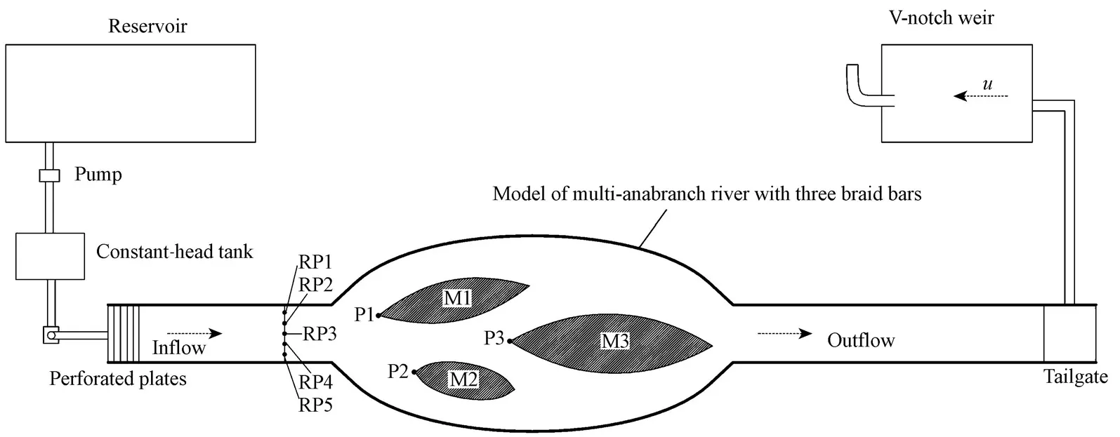
Fig. 1 Schematic layout of experimental model
The density of the tracer (salt solution) was maintained the same as that of the flume water by adding alcohol, and its concentration was measured with a multi-probe electrode conductivity meter. The data were saved in the computer automatically. Three probes, located in front of the tracer release position, were used to measure the background conductivity of flume water. Then, the measured conductivity value of other probes minus this background conductivity would be the actual conductivity induced by the tracer. The tracer was released from a circular pipe with an inner diameter of 1.4 cm, aligned parallel to the flume flow. The discharge orifice of the pipe was located at mid-depthH02, whereH0is the water depth of the main channel. Five transverse release positions, marked as RP1, RP2, RP3, RP4, and RP5 as shown in Fig. 1 and located 2.9 m upstream from the inlet section of the multi-anabranch reach, were adopted. The distances (d) from the five positions to the left bank of the upstream main channel were: 1/6B, 1/3B, 1/2B, 2/3B, and 5/6B, respectively, whereBis the width of the upstream main channel. The flow rate of the tracer was 50 L/h in the experiment.H0was kept at 6.0 cm. The multi-functional velocity instrument, developed by the Nanjing Hydraulic Research Institute, was used to measure the velocity.
In order to determine the pollutant concentration distribution in each branch, measured data at 20 cross-sections (Fig. 2) were acquired. The number of vertical profiles for concentration measurements along the cross-section in each branch varied according to the width of the branch. There were four points in each vertical line for concentration measurements.
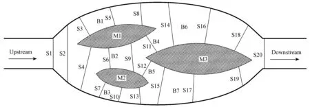
Fig. 2 Locations of measurement cross-sections
3 Results and discussion
3.1 Planar flow field characteristics
The water current from upstream flows into branches B1, B2, and B3. When the water current in branch B2 passes the braid bar M3, it flows into branches B4 and B5. Then, the water currents in branches B1 and B4 converge into branch B6. The water currents in branches B3 and B5 converge into branch B7. Finally, the water currents in branches B6 and B7 merge into the outlet.
In order to investigate the effect of different upstream discharge values (Q) on the velocity distribution in each branch, five upstream discharges were adopted: 2 L/s, 3 L/s, 4 L/s, 5 L/s, and 6 L/s. The non-dimensional longitudinal velocityu*is defined as, whereuis the longitudinal velocity, andmaxuis the maximum longitudinal velocity. The non-dimensional depthh*is defined ashH0, wherehis the water depth at the measurement point.b*is defined as, wherebis the distance from the measurement point to the left end of the section determined by looking downstream.
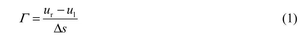
Longitudinal velocities at two arbitrary adjacent vertical lines at each section are respectively denoted asul(at the left side) andur(at the right side), as determined by looking downstream. The distance between the two adjacent vertical lines is denoted as Δs.Then, the lateral velocity gradient (Γ) for each section in each branch can be calculated by th e following equation:
The planar distributions ofu*in the surface layer (h*=0.80), the middle layer (h*=0.38), and the bottom layer (h*=0.22) forQ= 4 m/s3are shown in Fig. 3. The lateral variations of the velocity gradient for each section in each branch in the surface layer and the bottom layer forQ= 4 m/s3are shown in Fig. 4 and Fig. 5, respectively.
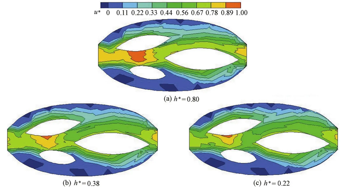
Fig. 3 Distributions of non-dimensional longitudinal velocities in three layers forQ= 4 L/s

Fig. 4 Lateral variation of velocity gradient for each section in each branch in surface layer forQ= 4 L/s
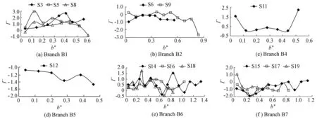
Fig. 5 Lateral variation of velocity gradient for each section in each branch in bottom layer forQ= 4 L/s
It can be seen from Fig. 3, Fig. 4, and Fig. 5 that flow structure is different in each of the seven branches. In addition, flow patterns are different in the surface and bottom layers. Flowvelocities in branch B1 decrease sharply to 0.11 from the right bank to the left bank. Due to water inertia and abrupt transition at the convergence of the main channel and the multi-anabranch reach, flow velocities in branch B1 are smaller than those in branch B2. Velocities in branch B2, which are the greatest of the seven branches, gradually diminish from the left bank to the right bank, and decrease to 0.33 near the right bank. Because the diversion point P2 of braid bar M2 is located outside the mainstream in the multi-anabranch reach, branch B3 is the unique branch with the flow velocity of zero among the seven branches. Velocities in branch B4 gradually decrease from the right bank to the left bank. Contours near the right bank in branch B5 are dense and velocity variation amplitudes per unit length are great. Flow velocities increase gradually from the left and right banks to the main channel centerline in the multi-anabranch reach. Flow velocities at one side near the braid bar are greater than those at another side near the bank in branches B1, B6, and B7. Flow velocities in the outlet area of branch B6 are larger those that in the outlet area of branch B7.
The velocity gradient (Γ) in the surface and bottom layers at three sections in branch B1 mainly ranges between 0 and 3.0. The value ofΓin the surface and bottom layers at two sections in branch B2 mainly ranges between −1 and 1. The measurement point in the surface layer of sections S11 and S12 with*0.2b= is a demarcation point. The value ofΓin the surface and bottom layers at three sections in branch B6 mainly ranges between 0 and 1.5. The value ofΓin the surface and bottom layers at three sections in branch B7 mainly ranges between 0 and −2.
Table 1 shows the percentage ratios of the discharges in branches B1, B2, and B3 to the upstream discharge for five upstream discharge conditions. The discharge in branch B2 accounts for about 80% of the upstream discharge because branch B2 is located in the primary flow direction. The discharge in branch B1 approximately accounts for 20% of the upstream discharge. As the diversion point P2 near branch B3 is located outside the primary flow, the discharge in branch B3 is equal to zero. It can be concluded that the percentage ratios of discharges in the three branches to the upstream discharge are determined by the distance from the diversion points P1, P2, and P3 to the mainstream centerline in the multi-anabranch reach .
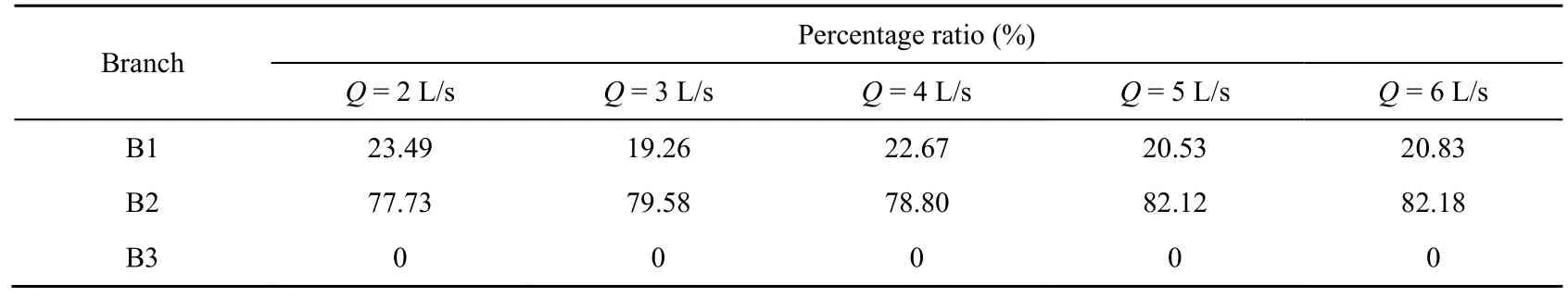
Table 1 Percentage ratios of discharges in three branches to upstream discharge for five discharge conditions
3.2 Concentration distribution in different branches
The non-dimensional pollutant concentrationC*is defined as, whereCis the pollutant concentration obtained from the measured conductivity, andCmaxis the maximumpollutant concentration. The pollutant mixing homogeneity extent (σ*) in each branch can be expressed as
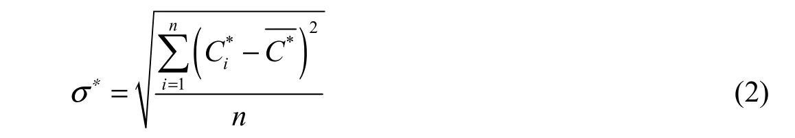
whereis the non-dimensional pollutant concentration ofith measurement point,is the average pollutant concentration of all measurement points in each branch, andnis the number of measurement points in each branch.
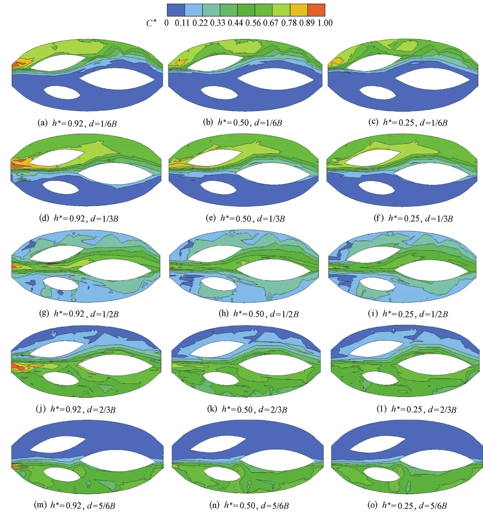
Fig. 6 Distributions ofC*in three layers for five release positions andQ= 4 L/s
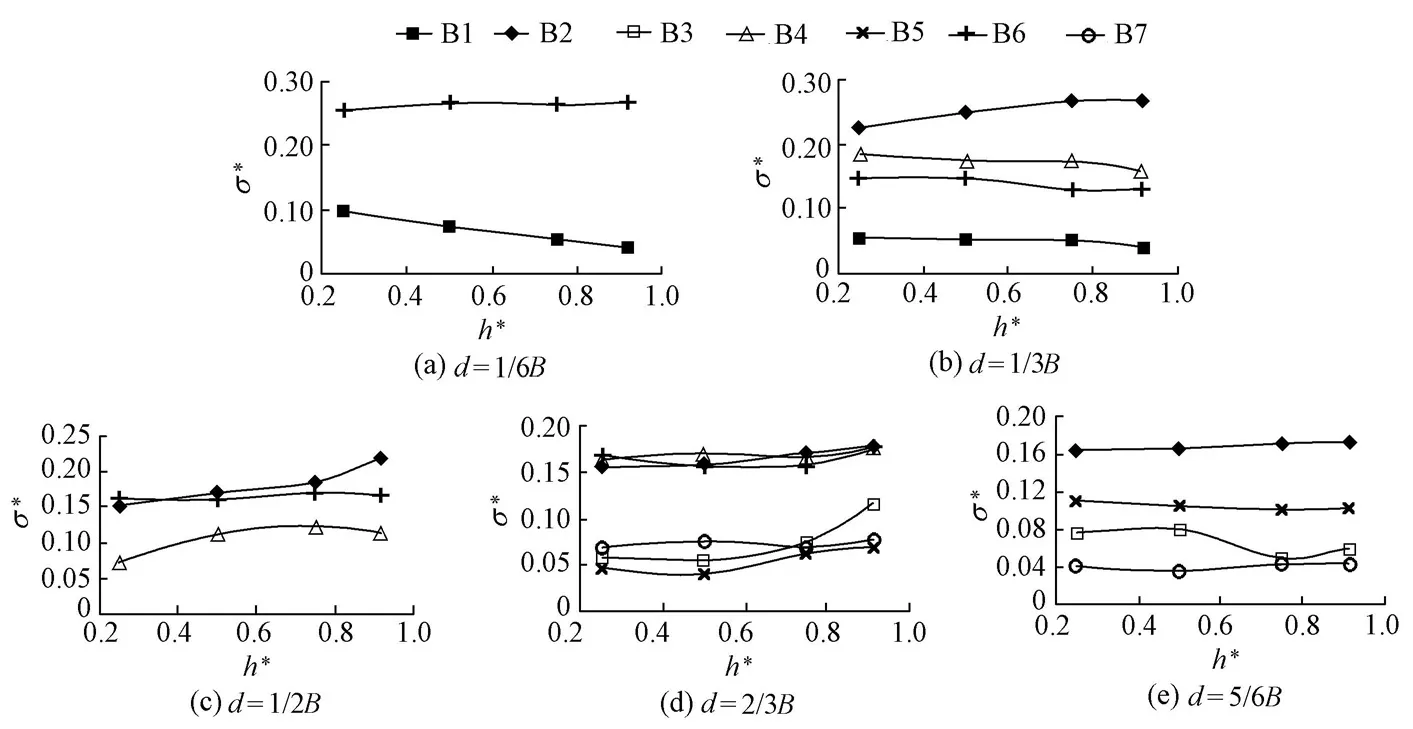
Fig. 7 Variations ofσ*withh*for five release positions andQ= 4 L/s
Fig. 6 shows the non-dimensional pollutant concentration distributions in the surface layer (h*=0.92), the middle layer (h*=0.50), and the bottom layer (h*=0.25) for five release positions andQ= 4 L/s. Fig. 7 shows the values ofσ*at four layers (h*= 0.25, 0.50, 0.75, 0.92) in each branch for five release positions andQ= 4 L/s. It can be seen from Fig. 6(a), Fig. 6(b), and Fig. 6(c) that, whend= 1/6B, the concentration contours near the braid bar M1 are dense, which indicates that the pollutants mostly flow into branch B1 and branch B6, and then reach the outlet. It can be seen from Fig. 7(a) that, whend= 1/6B,σ*in branch B6 changes little (around 0.15) from the bottom to the surface, whileσ*in branch B1 linearly decreases from the bottom to the surface, which means that pollutants mix more and more equably from the bottom to the surface.σ*in branch B6 is larger than doubleσ*in branch B1.
It can be seen from Fig. 6(d), Fig. 6(e), and Fig. 6(f) that, whend= 1/3B, the pollutants mostly flow into branches B1, B2, B4, and B6, ultimately reaching the outlet. It can be seen from Fig. 7(b) that, whend= 1/3B, with the increase ofh*,σ*varies slightly in branches B1, B4, and B6, while it linearly increases in branch B2.σ*in branch B2 is at the maximum for four branches, andσ*in branch B1 is at the minimum.
It can be seen from Fig. 6(g), Fig. 6(h), and Fig. 6(i) that, whend= 1/2B, the pollutants mostly flow into branches B2, B4, and B6, finally reaching the outlet. It can be seen from Fig. 7(c) that, whend= 1/2B,σ*in branch B2 is at the maximum for three branches, andσ*in branch B4 is at the minimum. With the increase ofh*,σ*gradually increases in branch B2, presents a parabolic distribution in branch B4, and varies little (around 0.15) in branch B6.
It can be seen from Fig. 6(j), Fig. 6(k), and Fig. 6(l) that, whend= 2/3B, pollutants mostly flow into branches B2, B3, B4, B5, B6, and B7, ultimately reaching the outlet. It can be seen from Fig. 7(d) that, whend= 2/3B,σ*in branches B2, B3, B4, B5, B6, B7 changes slightly.σ*in branches B2, B4, and B6 is greater than that in branches B3, B5, and B7.
It can be seen from Fig. 6(m), Fig. 6(n), and Fig. 6(o) that, whend= 5/6B, the pollutants mostly flow into branches B2, B3, B5, and B7, and then reach the outlet. It can be seen from Fig. 7(e) that, whend= 5/6B,σ*in branch B2 is at its maximum for the four branches.σ*in the four branches changes little with the increase ofh*.
It can be conclude from Fig. 7 that for five release positions,σ*in the most of brancheschanges little with the increase of the water depth, andσ*in branch B2 is the largest wh end= 1/3B. Whend= 1/3B,d= 1/2B, andd= 2/3B,σ*in branch B6 remains at about 0.15.
The percentage ratios of the pollutant fluxes in branches B1, B2, and B3 to the pollutant flux in the upstream main channel for five release positions and three upstream discharges,Q= 2 L/s, 4 L/s, and 6 L/s, are shown in Table 2. For different upstream discharges, the percentage ratios of the pollutant fluxes in branches B1, B2, and B3 are approximate at the same release position. The pollutant flux in branch B1 decreases as the release position moves from the left bank to the right bank. When the pollutants are released at RP1 and RP2, the pollutant flux in branch B1 is the maximum of the three branches. When the pollutants are released at RP3 and RP4, the pollutant flux in branch B2 is the maximum of the three branches. When the pollutants are released at RP5, the pollutant flux in branch B3 is the maximum of the three branches. The pollutant flux in branch B3 increases gradually as the release position moves from the left bank to the right bank. It can be inferred that the pollutant fluxes in branches B1, B2, and B3 vary with the release position. The diversion points and pollutant release positions jointly influence the flux allocation ratios in the three branches.

Table 2 Percentage ratios of pollutant fluxes in branches B1, B2, and B3 to pollutant flux in upstream main channel for different pollutant release positions and different upstream discharges
4 Conclusions
The mixing characteristics and transport processes of pollutants in a multi-anabranch river with three braid bars cannot be well understood due to the lack of measured data. A physical model experiment of a multi-anabranch river with three braid bars was carried out in the laboratory to explore the pollutant mixing characteristics in different branches. Major conclusions are as follows:
(1) Flow velocities from the left and right banks to the mainstream centerline in the multi-anabranch reach increase gradually. Flow velocities at one side near the braid bar are greater than those at another side near the bank in branches B1, B6 and B7. Branch B3 is a dead water region. Flow velocities in the outlet area of branch B6 are larger than those in the outlet area of branch B7. Flow velocities in branch B2 are the greatest of the seven branches. Flow velocities in the primary flow direction are larger than those in the other direction.
(2) For five release positions,σ*in the most of branches changes little with the increase of the water depth, andσ*in branch B2 is the largest whend= 1/3B. Whend= 1/3B,d= 1/2B, andd= 2/3B,σ*in branch B6 remains at about 0.15.
(3) The pollutant release positions are the main influencing factors in the pollutant transport process. The diversion points and pollutant release positions, rather than the flow discharge, determine flux allocation ratios in branches B1, B2, and B3 in a multi-anabranch river with three braid bars.
Baek, K. O., Seo, I. W., and Jeong, S. J. 2006. Evaluation of dispersion coefficients in meandering channels from transient tracer tests.Journal of Hydraulic Engineering, 132(10), 1021-1032. [doi:10.1061/(ASCE) 0733-9429(2006)132:10(1021)]
Bertoldi, W., Amplatz, T., Miori, S., Zanoni, L., and Tubino, M. 2006. Bed load fluctuations and channel processes in a braided network laboratory model.Proceedings of the International Conference on Fluvial Hydraulics-River Flow, 937-945. London: Taylor & Francis.
Bertoldi, W., Ashmore, P., and Tubino, M. 2009. A method for estimating the mean bed load flux in braided rivers.Geomorphology, 103(3), 330-340. [doi:10.1016/j.geomorph.2008.06.014]
Boxall, J. B., and Guymer, I. 2007. Longitudinal mixing in meandering channels: New experimental data set and verification of a predictive technique.Water Research, 41(2), 341-354. [doi:10.1016/j.watres. 2006.10.010]
Chau, K.W. 2000. Transverse mixing coefficient measurements in an open rectangular channel.Advances in Environmental Research, 4(4), 287-294. [doi:10.1016/S1093-0191(00)00028-9]
Deng, Z. Q., Singh, V. P., and Bengtsson, L. 2001. Longitudinal dispersion coefficient in straight rivers.Journal of Hydraulic Engineering, 127(11), 919-927. [doi:10.1061/(ASCE)0733-9429 (2001)127:11(919)]
Dietrich, W. E., and Smith, J. D. 1983. Influence of the point bar on flow through curved channels.Water Resources Research, 19(5), 1173-1192. [doi:10.1029/WR019i005p01173]
Gu, L., Hua, Z. L., Zhang, C. K., Chu, K. J., and Dai, W. H. 2011. Mixing characteristics and transport flux ratio of pollutants in braided rivers.Fresenius Environmental Bulletin, 20(9), 2315-2325.
Guymer, I. 1998. Longitudinal dispersion in a sinuous channel with changes in shape.Journal of Hydraulic Engineering, 124 (1), 33-40. [doi:10.1061/(ASCE)0733-9429(1998)124:1(33)]
Holly, F. M., Jr., and Yang, J. C. 1985. Numerical modelling of bed evolution in braided channel systems.Proceedings of the 1985 ASCE Hydraulics Division Specialty Conference on Hydraulics and Hydrology in the Small Computer Age, 807-814. New York: ASCE.
Hua, Z. L., Gu, L., and Chu, K. J. 2009. Experiments of three-dimensional flow structure in braided rivers.Journal of Hydrodynamics, Ser. B, 21(2), 228-237. [doi:10.1016/S1001-6058(08)60140-7]
Lane, S. N., and Richards, K. S. 1998. High resolution, two-dimensional spatial modelling of flow processes in a multi-thread channel.Hydrological Processes, 12(8), 1279-1298. [doi:10.1002/(SICI)1099-1085 (19980630)12:8<1279::AID-HYP615>3.0.CO;2-E]
Lu, Y. J., Wang, Z. Y., Zuo, L. Q., and Zhu, L. J. 2005. 2D numerical simulation of flood and fluvial process in the meandering and island-braided middle Yangtze River.International Journal of Sediment Research, 20(4), 333-349.
Navratil, O., Legout, C., Gateuille, D., Esteves, M., and Liebault, F. 2010. Assessment of intermediate fine sediment storage in a braided river reach (southern French Prealps).Hydrological Processes, 24(10), 1318-1332. [doi:10.1002/hyp.7594]
Nicholas, A. P., and Smith, G. H. S. 1999. Numerical simulation of three-dimensional flow hydraulics in a braided channel.Hydrological Processes, 13(6), 913-929. [doi:10.1002/(SICI)1099-1085 (19990430)13:6<913::AID-HYP764>3.0.CO;2-N]
Pittaluga, M. B., Repetto, R., and Tubino, M. 2003. Channel bifurcation in braided rivers: Equilibrium configurations and stability.Water Resources Research, 39(3), 1046-1059. [doi:10.1029/ 2001WR001112.]
Richardson, W. R., and Thorne, C. R. 1998. Secondary currents around braid bar in Brahmaputra River, Bangladesh.Journal of Hydraulic Engineering, 124(3), 325-328. [doi:10.1061/(ASCE)0733-9429 (1998)124:3(325)]
Richardson, W. R. and Thorne, C. R. 2001. Multiple thread flow and channel bifurcation in a braided river: Brahmaputra-Jamuna River, Bangladesh.Geomorphology, 38(3-4), 185-196. [doi:10.1016/S0169-555X(00)00080-5]
Salikov, V. G. 1989. Distribution of water discharges and current velocities in a braided channel.Hydrotechnical Construction, 23(2), 88-91. [doi:10.1007/BF01427932]
Seo, I. W., Lee, M. E., and Baek, K. O. 2008. 2D modeling of heterogeneous dispersion in meandering channels.Journal of Hydraulic Engineering, 134(2), 196-204. [doi:10.1061/(ASCE)0733-9429 (2008)134:2(196)]
Szupiany, R. N., Amsler, M. L., Parsons, D. R., Best, J. L., and Haydel, R. 2007. Comparisons of morphology and flow structure at two braid-bar confluences in a large river.Proceedings of the 5th IAHR Symposium on River, Coastal and Estuarine Morphodynamics, 807-814. London: Taylor & Francis.
Walsh, J., and Hicks, D. M. 2002. Braided channels: Self-similar or self-affine?Water Resources Research, 38(6), 181-186. [doi:10.1029/2001WR000749]
Zanoni, L., Bertoldi, W., and Tubino, M. 2007. Spatial scales in braided networks: Experimental observations.Proceedings of the 5th IAHR Symposium on River, Coastal and Estuarine Morphodynamics, 201-207. London: Taylor & Francis.
Zeng, Y. H., Huai, W. X., and Guymer, I. 2008. Transverse mixing in a trapezoidal compound open channel.Journal of Hydrodynamics,Ser. B, 20(5), 645-649. [doi:10.1016/S1001-6058(08)60107-9]
(Edited by Yan LEI)
This work was supported by the National Basic Research Program of China (973 Program, Grant No. 2008CB418202), the National Natural Science Foundation of China (Grants No. 50979026 and 51179052), the National Key Technologies R&D Program of China (Grant No. 2012BAB03B04), the Special Fund for Public Welfare Industry of the Ministry of Water Resources of China (Grant No. 201001028), the “Six Talent Peak” Project of Jiangsu Province (Grant No. 08-C), and the Fundamental Research Funds for the Central Universities (Grant No. 2010B15514).
*Corresponding author (e-mail:zulinhua@hhu.edu.cn)
Sep. 7, 2012; accepted Apr. 11, 2013
 Water Science and Engineering2013年3期
- Water Science and Engineering的其它文章
- Present and future of hydrology
- Characteristics of phosphorus adsorption by sediment mineral matrices with different particle sizes
- Joint probability distribution of winds and waves from wave simulation of 20 years (1989-2008) in Bohai Bay
- Optimized operation of cascade reservoirs on Wujiang River during 2009-2010 drought in southwest China
- Towards full predictions of temperature dynamics in McNary Dam forebay using OpenFOAM
- Effectiveness of inhibitors in increasing chloride threshold value for steel corrosion