STABILITY OF A PREDATOR-PREY SYSTEM WITH PREY TAXIS IN A GENERAL CLASS OF FUNCTIONAL RESPONSES∗

M.YOUSEFNEZHADDepartment of Mathematical Sciences,Sharif University of Technology,Tehran,IranE-mail:yousefnezhad@mehr.sharif.irS.A.MOHAMMADIDepartment of Mathematics,College of Sciences,Yasouj University,Yasouj,75918-74934,IranE-mail:mohammadi@yu.ac.ir



STABILITY OF A PREDATOR-PREY SYSTEM WITH PREY TAXIS IN A GENERAL CLASS OF FUNCTIONAL RESPONSES∗

M.YOUSEFNEZHAD
Department of Mathematical Sciences,Sharif University of Technology,Tehran,Iran
E-mail:yousefnezhad@mehr.sharif.ir
S.A.MOHAMMADI†
Department of Mathematics,College of Sciences,Yasouj University,Yasouj,75918-74934,Iran
E-mail:mohammadi@yu.ac.ir

AbstractIn this paper,a di ff usive predator-prey system with general functional responses and prey-tactic sensitivities is studied.Providing such generality,we construct a Lyapunov function and we show that the positive constant steady state is locally and globally asymptotically stable.With an eye on the biological interpretations,a numerical simulation is performed to illustrate the feasibility of the analytical findings.

Key wordspredator-prey;global stability;steady state;Lyapunov function

2010 MR Subject Classi fi cation35K57;35K55;92B05

∗Received January 5,2015;revised March 16,2015.

†Corresponding author:S.A.MOHAMMADI.

1 Introduction

Typical mathematical questions in the theory of reaction-di ff usion equations deal with existence of solutions,global boundedness of solutions by means of maximum and invariant region method,large time asymptotic,traveling waves,and geometry and topology of attracting sets,singular limits etc.The maybe most essential mathematical problem in the study of reaction-di ff usion equations refers to the stability properties of the reaction-di ff usion system under consideration[1-6].

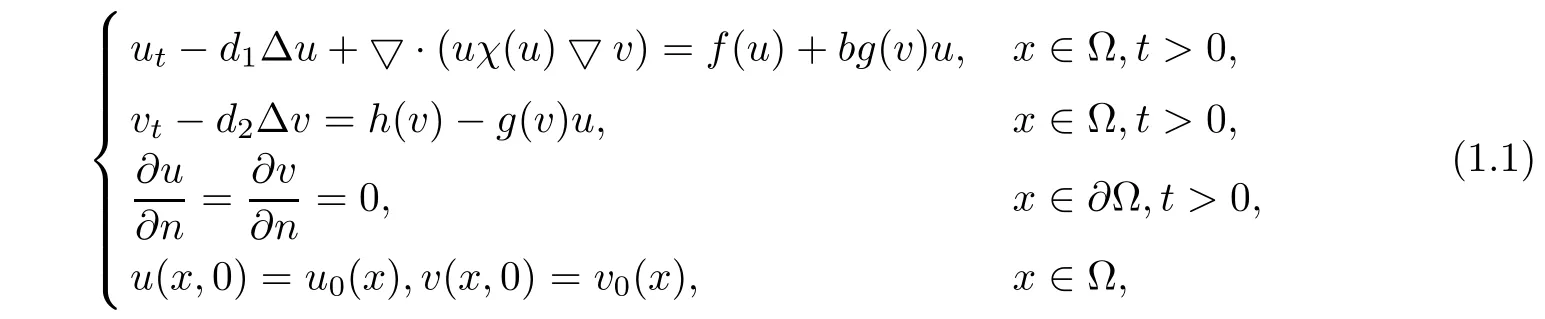
In this study we discuss the question of the stability of the unique positive constant solution of the following reaction-di ff usion systemwhere Ω is a bounded domain in RN,with su ffi ciency smooth boundary∂Ω and outer unit normal n.Equation(1.1)is known as a predator-prey system and in this equation u(x,t)and v(x,t)denote the predator and the prey population densities at position x and time t.In the model above,d1,d2＞0 are the di ff usion rates of predator and prey,respectively,and b＞0 is the conversion rate from prey to predator.The function g(v)is called the functional response of the predator to the prey and describes the change in the rate of exploitation of the prey by a predator as a result of a change in the prey density.Indeed,the growth of the predator is enhanced in the presence of the prey by an amount proportional to the number of prey.Thus,the functional response can be interpreted as the consumption rate of the prey by an individual predator.The functionis the logistical growth rate of prey where r＞0 is the natural growth of prey and K＞0 is the carrying capacity.We take the mortality rate of the predator in the quadratic form f(u)=−au2where a is a positive constant[7].

System(1.1)proposed by Ainseba,Bendahmane and Nousair in[8]has an interesting point.In addition to the random di ff usion of predators and the prey,the spatial-temporal variations of the predator’s velocity are directed by prey-taxis.Prey-taxis is de fined as the movement of predators controlled by the prey density.This means that predators in area-restricted search tend to move towards areas with high food abundance to increase the e ffi ciency of foraging.The term uχ(u)∇v gives the velocity by which predators move up to the gradient of the prey where χ(u)denotes their prey-tactic sensitivity.Other studies measuring characteristics of individual movement support the mechanism of prey-taxis.For instance,a chemotaxis-haptotaxis model of cancer invasion of tissue includes the prey-taxis mechanism.The migration of cancer cells is biased towards a gradient of the di ff usible matrix degrading enzymes,the prey-taxis mechanism,which is referred to as chemotaxis[9].

The mathematical investigation of chemotaxis models,typical models include the mechanism of prey-taxis,started with a work of Patlak[10]and developed by the papers of Keller and Segel.They introduced a model to study the aggregation of Dictyostelium discoideum due to an attractive chemical substance[11,12].We refer to[13]for a review of the beginning of the researches on the Keller-Segel model.Recently,there have been three major extensions of the Keller-Segel model.The first one takes into account a nonlinear chemotactic sensitivity function[14,15].The second extension includes a nonlinear di ff usion term,[14,16],and the third one incorporates a logistic term,see[17,18].

For the linear form of mortality rate of the predator,f(u)=−au,in[8],authors proved the existence and uniqueness of weak solutions to system(1.1).In case that the function f has the linear form,the global stability of the positive steady state solution of(1.1)with the speci fi c prey-tactic sensitivity(1.2)and Holling-type II functional response was proved in[19].

In this paper,we study the asymptotical stability of the positive steady state of system(1.1)in a general framework.The functional response g belongs to a large class of functions and it can take a complicated nonlinear form.Indeed,this is a generalization of well known functional responses which depend on the density of the prey.The mortality rate of the predator is considered in a quadratic form.Motivated by the volume- fi lling mechanism,χ is assumed to bein[19],where α,umare positive constants.It is important to note that in this paper χ is of the general form that it should only satisfy following conditions

(i)χ(u)=0 for all u≥um,

(ii)|χ(u)|≤B1and|χ′(u)|≤B2for all u≥0,

where B1,B2are positive constants.Assumption(i)has a biological interpretation[8]:the predators stop to accumulate at a given point of Ω after their density attains the certain threshold value umand the prey-tactic cross di ff usion η(u):=uχ(u)vanishes identically when u≥um.

Providing such generality,we derive a suitable Lyapunov function and prove that the positive constant steady state is locally and globally asymptotically stable.Finally,a numerical simulation is performed to illustrate the feasibility of the analytical results.

2 Global Stability

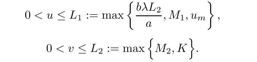
In this section we examine the stability of positive constant solutions of system(1.1)for functional response g(v).Let M1,M2be positive constants such that

Henceforth,we assume that

(iii)0＜u0(x),0＜v0(x).

Throughout this section,we consider a generalized function g where

(iv)g(v)≥0 for all v∈[0,+∞),and g′(v)＞0 for all v∈(0,+∞),

(v)bg2(v)＜ah(v)for all

(vi)g(0)=0 and g(v)is Lipschitz with the Lipschitz coeffi cient λ,i.e.,|g(v1)−g(v2)|≤λ|v1−v2|for all v1,v2∈[0,+∞),

where λ is a positive constants.

Invoking(vi),we see that

Before proving the main result of this section,we need the following technical assertion.

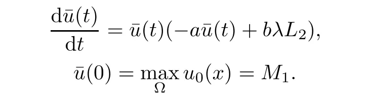
Lemma 2.1Assume that(u,v)is a solution of system(1.1),then we have

ProofApplying the maximum principle[20]and assumption(iii),it can be deduced

In addition,in view of(iv),

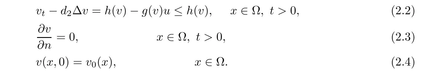
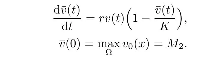
is a sub-solution to the problem(2.2)-(2.4).Hence by the maximum principle

Taking into account v≤L2,(2.1)and(2.1),for u≥um,we have

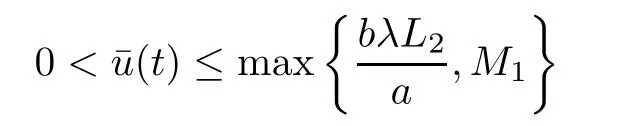
is a sub-solution to the problem(2.5)-(2.7).Again,by the maximum principle,if u≥umthen we have

and therefore,in both cases we get

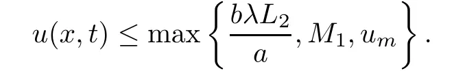
This completes the proof.

Now,we return to the main result.The equilibrium points of system(1.1)are solutions of the following equations

It is easy to check that there are precisely three equilibrium states:the trivial states(0,0),(0,K)and the unique positive steady state(u∗,v∗)which is derived in the following calculation.We know that

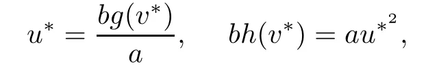
and so,ah(v∗)=bg2(v∗).It is clear that from assumptions(iv)and(v),the following equation

has unique solution 0＜v∗＜K.

We are interested in the stability of the unique positive steady state(u∗,v∗).From(2.1),we have

Assume 0=µ0＜µ1＜···＜µk＜···denote the eigenvalues of−∆in Ω under the homogeneous Neumann boundary condition.Let us first consider the local stability of(u∗,v∗).

Theorem 2.2Let

then the positive constant steady state(u∗,v∗)is locally asymptotically stable.

ProofSet z∗=(u∗,v∗),the linearization of(1.1)at z∗can be expressed by

where z=(u,v)T,

and

Also,by simple calculations,we get

Consider the following eigenvalue problem

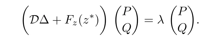
Then,λ is an eigenvalue of D∆+Fz(z∗)if and only if λ is an eigenvalue of the matrix Wk= −µkD+Fz(z∗)for each k≥0.The characteristic polynomial of Wkis given by

where

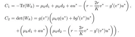
Now,by(2.9)and(iv)we have C1,C2＞0,and so the characteristic roots of(2.10)have negative real parts which yields the desired result.

Now,we address the global stability of the positive steady state(u∗,v∗)using Lyapunov techinques.

then the positive constant steady state(u∗,v∗)is globally asymptotically stable.

ProofLet(u(x,t),v(x,t))be a solution of(1.1).In order to prove the theorem,it is su ffi cient to construct a suitable Lyapunov function.For this purpose,we de fi ne the following Lyapunov function

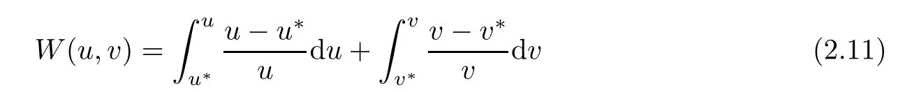
and

Using a simple calculation,it follows that

where

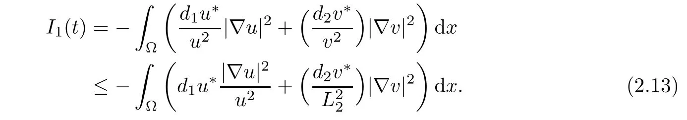
From Lemma 2.1,we have 0＜v≤L2,and due to the Neumann boundary condition,we observe

Because of the Neumann boundary condition,(i)and(ii),we see that

Furthermore,from assumption(vi),

Moreover,h(v∗)−g(v∗)u∗=0,which yields

and so

Then,from(2.16),(2.8)and assumption(vi),we have

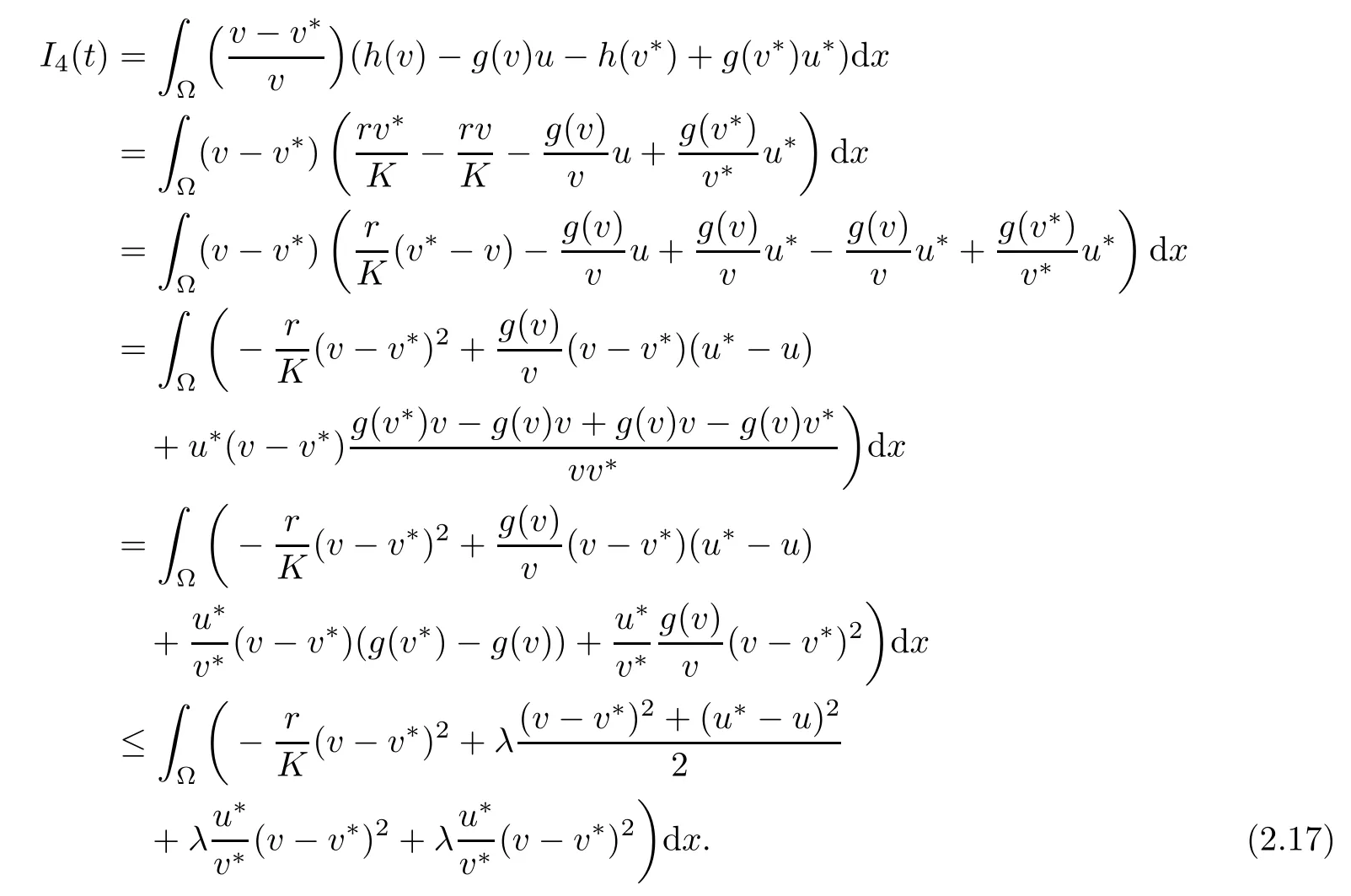
Thus,from(2.12)-(2.17)we obtain

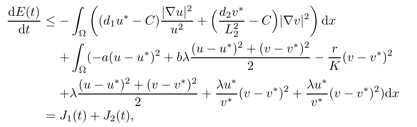
where

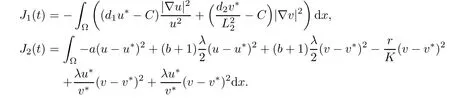
From(A2),we have J1(t)≤0.Additionally,from(2.8),

Applying(A1),we have J2(t)≤0.Thus

3 Numerical Simulation

In this section we provide a numerical result in two dimension implemented for the simulation of prey-predators interactions.With an eye on the biological interpretations,the numerical simulation illustrates the feasibility of the analytical findings.

The habitat Ω is surrounded by an ellipse with the major axis from(−2,0)to(2,0)and the minor axis from(0,−1)to(0,1).The zero- fl ux boundary conditions in(1.1)mean that no individuals cross the boundary of the habitat.The initial distribution of the predators is a vertical band of width 1 and height 1.6.The function u0equals 0.4 in the band and is zero elsewhere,see Fig.1(a).The preys are distributed initially in a horizontal band of width 0.8 and height 2.8.The function v0equals 0.5 in the band and is zero elsewhere,see Fig.1(b).

In the example we take the following ecological parameter

Although the result of the previous section is valid for the usual functional responses,we consider the functional responses g and the prey-tactic sensitivity χ in the following nonlinear

forms

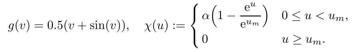
Indeed,this complicated forms show the generality of the analytical findings.It is easy to check that functions g and χ with above parameters satisfy the conditions of Section 2.

Fig.1 Initial distribution of the predators and preys

The calculations are based upon the standard finite element Garerkin method with the time step∆t=0.01.

In Figs.2-5,we can see the spatial and temporal behavior of the interacting species.First,the predator population increases in the initial coincidence domain while we observe the preys escape toward the boundary of the horizontal band.Due to the higher di ff usion,the preys continue the movement toward the boundary of the habitat.This give rise to the attraction of predators toward the boundary of the habitat because of the prey taxis effect.Indeed,we can see the direct movement of the predator toward the prey regarding the the effect of the prey taxis and the di ff usion.The effect of the prey taxis vanishes when the population prey is homogenous in the habitat since the gradient vanishes.The two population interact and the the prey population increases but it is controlled by the predators populations.At last,two population reach the positive steady state u∗=0.19 and v∗=0.40.Indeed,two population interact and grow or decay until the whole region is at populations’s coexistence steady state.

Fig.2 Dynamics of the predator population

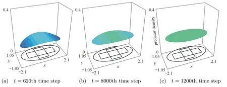
Fig.3 Dynamics of the predator population

Fig.4 Dynamics of the prey population

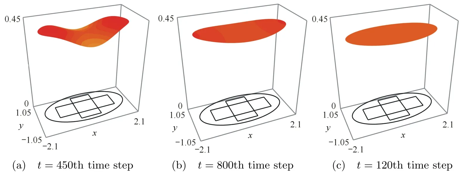
Fig.5 Dynamics of the prey population

4 Conclusion

This paper extends well-known predator-prey system with prey-taxis to a general one with quadratic mortality rate of the predator.The functional response g can take a complicated nonlinear form and it should satisfy conditions(iv)-(vi).The prey-tactic sensitivity is not restricted to the simple form(1.2).Indeed,it is of the general form such that it should onlyverify conditions(i)-(ii).In view of such generality,we have addressed the question of the stability of the unique positive steady state.At first,the local stability of the positive constant steady state have been proved.Next,we obtain a sharper result,the global stability,employing Lyapunov techniques.

The spatial and temporal behavior of the interacting species have been shown by a numerical result in two dimension.Two population interact until they reach the steady state.

It would be interesting if the existence of non-constant steady states of such general model are investigated in the future studies.

References

[1]Smoller J.Shock Waves and Reaction Di ff usion Equations.Grundlehren Series 258.Springer-Verlag,1982

[2]Qin Y,Li H.Global existence and exponential stability of solutions to the quasilinear thermo-di ff usion equations with second sound.Acta Mathematica Scientia,2014,34B(3):759-778

[3]Wang S L,Feng X L,He Y N.Global asymptotical properties for a di ff used HBV infection model with CTL immune response and nonlinear incidence.Acta Mathematica Scientia,2011,31B(5):1959-1967

[4]Jin Z,Ma Z E,Han M A.Global stability of an SIRS epidemic model with delays.Acta Mathematica Scientia,2006,26B(2):291306

[5]Li W T,Wang Y,Zhang J F.Stability of positive stationary solutions to a spatially heterogeneous cooperative system with cross-di ff usion.Elec J Di ff er Equ,2012,223:1-18

[6]Yu X,Sun F.Global dynamics of a predator-prey model incorporating a constant prey refuge.Elec J Di ff er Equ,2013,04:1-8

[7]Baurmann M,Gross T,Feudel U.Instabilities in spatially extended predator prey systems:Spatio-temporal patterns in the neighborhood of Turing-Hopf bifurcations.J Theor Biol,2007,245:220-229

[8]Ainseba B E,Bendahmane M,Noussair A.A reaction-di ff usion system modeling predator-prey with preytaxis.Nonlinear Anal Real World Appl,2008,9:2086-2105

[9]Tao Y,Cui C.A density-dependent chemotaxis-haptotaxis system modeling cancer invasion.J Math Anal Appl,2010,367:612-624

[10]Patlak C S.Random walk with persistence and external bias.J Theor Biol,1971,30:235-248

[11]Keller E F,Segel L A.Initiation of of slide mold aggregation viewed as an instability.J Theor Biol,1970,26:399-415

[12]Keller E F,Segel L A.Traveling bands of chemotactic bacteria:a theoretical analysis.J Theor Biol,1971,30:235-248

[13]Keller E F.Assessing the Keller-Segel model:how has it fared//Biological Growth and Spread.Lect Notes Biom,38.(Proc Conf Heidelberg,1979).Springer-Verlag,1980:379-387

[14]Cieslak T,Morales-Rodrigo C.Quasilinear nonlinear non-uniformly parabolic-elliptic system modelling chemotaxis with volume fi lling effect:existence and uniqueness of global-in-time solutions.Topol Methods Nonlinear Anal,2007,29:361-382

[15]Hillen T,Painter K.Global existence for a parabolic chemotaxis model with prevention of overcrowding.Adv Appl Math,2001,26:280-301

[16]Kowalczyk R,Szymaska Z.On the global existence of solutions to an aggregation model.J Math Anal Appl,1971,30:235-248

[17]Tao Y.Global existence of classical solutions to a combined chemotaxis-haptotaxis model with logistic source.J Math Anal Appl,2009,354:60-69

[18]Tello J T,Winkler M.A chemotaxis system with logistic source.Comm Partial Di ff erential Equations,2007,32:849-877

[19]Li C,Wang X,Shao Y.Steady states of a predator-prey model with prey-taxis.Nonlinear Anal,2014,97:155-168

[20]Ladyzenskaja O A,Solonnikov V A,Ural’ceva N N.Linear and Quasi-Linear Equations of Parabolic Type.Amer Math Soc Transl 23.Providence,RI:Amer Math Soc,1968

[21]LaSalle J,Leftschetz S.Stability by Lyapunov’s Direct Method.New York:Academic Press,1961