A model offlow separation controlled by dielectric barrier discharge

Mohammadreza BARZEGARAN,Amirreza KOSARI

Faculty of New Science and Technologies,University of Tehran,Tehran 1417466191,Iran

A model offlow separation controlled by dielectric barrier discharge

Mohammadreza BARZEGARAN,Amirreza KOSARI*

Faculty of New Science and Technologies,University of Tehran,Tehran 1417466191,Iran

Flow separation,as an aerodynamic phenomenon,occurs in specific conditions.The conditions are studied in a wind tunnel on different airfoils.The phenomenon can be delayed or suppressed by exerting an external momentum to the flow.Dielectric barrier discharge actuators arranged in a row of 8 and perpendicular to the flow direction can delay flow separation by exerting the momentum.In this study,a mathe matical model is developed to predict a parameter,which is utilized to represent flow separation on an NACA0012 airfoil.The model is based on the neurofuzzy method applied to experimental datasets.The neuro model is trained in different flow conditions and the parameter is measured by pressure sensors.

1.Introduction

Many aerodynamic phenomena can be demonstrated in both experimental and computational flow dynamics;however,based on the nature of experimental and computational flow,results might be slightly different.This is a great advantage if the re is a way to make a connection between experimental and computational methods.One of the best examples is‘CFD in the loop” modeling.1Learning algorithms are one of the methods of modeling.The method represents a mathe matical model based on experiments carried out in specific situations,let’s say a state space.A state space describes setting of input parameters in an experiment.The mathe matical model is credible in the state space.Some learning methods can also predict the behavior outside the state space.These models predict the behavior of a system like an oracle.2Experimental flow dynamics needs state space declaration based on the goal of the experiment and nature of the phenomenon.By contrast,computational flow dynamics is mostly based on flow behavior simulation utilizing governing equations on flow,such as Navier-Stokes.The equations should be generalized in a desired space.The equations might need linearization in subspaces,both stable and unstable subspaces,and generalize simplified differential equations.3In some conditions,linearization is not suitable and might make the equations invalid.In the se conditions,additional correlation methods are preferable.For more complex dynamics,the same procedures for linearizing ordinary differential equations utilizing a correlation matrix are considered.4

On the other hand,separation is an aerodynamic phenomenon that occurs in many engineering applications.5The phenomenon is sometimes desired and the goal is to make it happen,but sometimes,it is undesirable and should be controlled.The control process of an aerodynamic phenomenon is another field of science called flow control.Flow control is divided into two distinct divisions,open-loop flow control and closed-loop flow control.There are various control parameters involved in separation.6By controlling each of the se parameters or combination of the se parameters,various solutions are presented for the separation control problem.An open-loop control solution is very co7mmon,which is mostly carried out with mechanical actuators.An example is the flaps utilized in airplanes during take-off and landing phases to control separation and augmentation of the lift force.The flaps

8delay separation by exerting a momentum to the flow.Open-loop control doesn’t have adequate control authority due to the fact that the re is no feedback from the system.Closed-loop flow controlfocused on enhancing control authority is presented.There are different types of actuators that can be utilized in closed-loop control.Using dielectric barrier discharge actuators is a method for flow control with desirablefeatures in some aspects.6Many researchers have studied active flow control utilizing dielectric barrier discharge actuators.Active separation control leads to a great enhancement in the performance of air vehicles.

In order to actively control an a9erodynamic phenomenon,the flow system should be identified.Several studies have been carried out exclusively to identify the dielectric barrier discharge model.The model is mostly numerical,like those expressed by Mohammadreza10and Sjoberg et al.11The prior identifications need to know the physics of every part of the system,which might be unknown.A slight change in the model of one part can cause the system to be misidentified.This leads to the use of techniques where no precise knowledge of the physics of the system is needed.Such modeling of a system is carried out by different methods.Neural network is a method based on the history of the system’s behavior.1The Local Linearization Model of tree(LoLiMot)method and the Nonlinear AutoRegressive with eXogenous(NARX)method are two common methods of modeling neural networks.5By defining an appropriate state space,the LoLiMot and NARX methods offer a model that not only perfectly fits the system but also is attached to the knowledge of the system’s physics.The methods have a wide range of applications from Single Input Single Output(SISO)to Multi Input Multi Output(MIMO)systems.5Several recent researches on activeflow control are based on the se methods.A similar method wasutilized by Tian etal.to identify separation on NACA0025.In the study,model definition and separation identification(usage of the model)are simultaneous.The method presented is called online.12The NARX method was used by Dandois et al.to develop a model for those with unsteady flow.Separation control with synthe tic jet actuators utilizes the developed method.5It is obvious that model definition and usage of the model are not simultaneous.These types of methods are called of fline.

In the present study,a flow model which is defined as of fline is utilized to identify separation.Once separation is identified,an appropriate momentum is exerted to flow by Dielectric Barrier Discharge(DBD)actuators to suppress separation.The appropriate momentum is calculated according to the system’s history.A modified LoLiMot is utilized in model definition.

A LoLiMot tries to fit a linear function in subspaces of a state space and present a model by combining linear functions.A modified Takagi-Segno LoLiMot method was presented by Kalhor et al.to reduce iteration and make the model more accurate.13The modified model was utilized in the presented flow modeling.

In this study,the modified LoLiMot method is utilized to identify the flow separation behavior of NACA0012 airfoil affected by open-loop momentum exertion of dielectric barrier discharge arrays.An array of 8 dielectric barrier discharge stimuli is utilized to control flow separation.The modified LoLiMot model generates an Multi Input Single Output(MISO)model for flow separation and actuators array in open-loop momentum exertion.The goal is to present a simple nonlinear model of the system which can be utilized in controller design for flow control.

2.Flow model and control law

As mentioned earlier,a modified LoLiMot method is utilized in this study to develop a model for flow behavior.In order to train the modified LoLiMot method,a valid state space should be defined.The state space definition is based on the knowledge of the flow system.For the first step,the modified LoLiMot method is explained.

Takagi,Segno,and Kank havecarried outseveral researches in the field of neural networks.Their researches led to a learning algorithm based on fuzzy logics.13The algorithm follows a pattern to optimize speed.The pattern is one of the most speed-optimal learning patterns.Creating flexible subspaces makes the Takagi algorithm fast enough to be utilized in speed-sensitive applications.14

The method creates membership functions so as to convert datasets in a subspace into a series of blocks.This means that each of the subspaces is divided into series of blocks.The algorithm assumes that each newly created block is a subspace and repeats the procedure.The algorithm repeats the same procedure until a predefined condition is met.In each block,the algorithm tries to fit a linear function.The step is successful if the re is a linear function fitted in each block.In the function fitting stage,the fitted function might have a slight stability error.

The stop condition for the subspace creation algorithm is the two criteria discussed above,linear function fitted in each block and predefined stable error for the fitted function.14In the final stage,the re is a linear function in each of the subspaces created.In other words,it can be said that the algorithm is a locally linearized method.A function is defined by accumulation of the locally linearized functions.The domain of the defined function is split into various subspaces in which the defined functions are linear.In order to meet the stop condition,a game rule tries to optimize the local linear function creation and subspace creation.Along with the subspace division process,the game rule controls the function fitting so as to minimize the error.The game rule comprises different algorithms such as merge,split,and division to create a new game rule in each block.This means that in each of the subspaces,the re is a game rule.

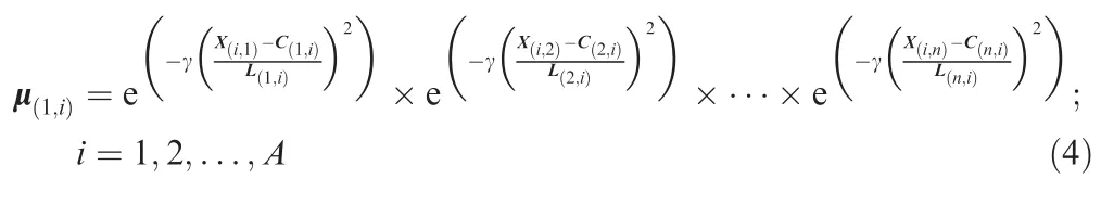
The process of creating the game rule continues until the index error,from the first step to the last step,experiences no serious loss.It is obvious that the algorithm looks like a tree.It starts from the trunk(state space)and divides into series of branches(subspaces),and each branch is divided into other series of branches.Branches with a serious error index are cut.Therefore,the re are only a few paths left from trunk to some branches.Branches with the least error are the desired paths.This is the reason why the method is called a tree model.The game rule checks the loss in an error index.Any serious loss in an error index demonstrates that the re is a great gap between the main subspaces and the current ones.The great gap between subspaces demonstrates that locally linearized functions in subspaces are highly angled in the border of two subspaces.The high angle means that the data points in subspaces are not united and this is due to the creation of subspaces.Game rules and subspaces creation according to membership functions is illustrated in Fig.1.14The M index demonstrates the current step where subspaces and game rules are created.Number of data blocks arefed to the algorithm represented by b and superscripted with 1 to N.In each step of the algorithm a subspace denoted by C is created and indexed to M which is mentioned before,representing current step of the algorithm.LLM illustrates the game-rule controlling subspaces by means of cost function φ to form a locally linearized function of^yifor each subspaces from 1 to M.Finally,the output^y forms by summation of^yifrom 1 to M.

Thefinal function takes x∈Rn(an array of n elements)as the input and y∈R is the output.The model represents an MISO system.The Takagi algorithm defines a general algorithm for neural networks.The method utilized here is a modification of the algorithm presented by Kalhor et al.Here,the modified LoLiMot is changed in a way that fits our usage.The data fed to the algorithm are in the form of（x1，x2，x3，...，xn，y）.

In order to train the model,a series of data points should befed to the learning algorithm.More data points mean more accurate models.The number of datasets fed to the system is denoted by Q.The pairs of input-output datasets are（xq，yq），q=1，2，...，Q.On the other hand,each dataset has an observer which observes the nonlinear function;the refore,q represents observers and the number of datasets.The algorithm will be repeated A times,which represents the iteration which is denoted by i.For each iteration,a cost function is defined to represent the error.The cost function θ should be minimized.The function is calculated by a weighted least square technique.The cost function is illustrated as

Fig.1 Game rules and subspaces creation in learning algorithm.14

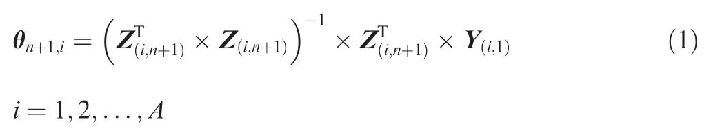
The cost function is a function of inputs and output of the system.In the equation of calculation of θ,the matrice Z is defined as a matrice with A rows and n+1 columns.The matrice is illustrated as

Each row of matrice Z represents a dataset related to each iteration.On the other hand,the first n columns of the matrice represent inputs and the last column represents the output of the system.The last column of matrice Z is described as Y.The definition of matrice Y is illustrated as

There are two options for the algorithm to set.The first option is the number of neurons.The final error of the system is decreased as the neuron number is increased.An increase in the neuron number takes more calculation time.There is a trade off between calculation time and final error.The second option in the algorithm is the divergent factor denoted by γ.The divergent factor controls the loss of an error index in game rule creation.The output of the algorithm is C,L,θ and φ matrices.

Matrice C represents the final subspaces,which completely fits the stop condition of the algorithm;the refore,the dimension of matrice C is n×A.The length of each subspace is stored in a related element of matrice L.As mentioned earlier,matrice θ represents the cost function values.In order to form the final locally linearized function,some mathematical operations should be carried out.For the first step,matrice μ is defined as

The dimension of matrice μ is 1 × A.Matrice μ,defined earlier,is utilized to form matrice φ.Matrice φ,with a dimension of 1×A,is defined as

Matrice φ defined here and the matrice cost function θ which is defined before are utilized to define a coefficient matrice B.Matrice B is a （n+1）× 1 size matrice.The B matrice is defined as

Each element of matrice B is a coefficient for an input;the refore,by using x as the input,the final locally linearized function which describes the system behavior becomes

The mathe matical relation defined here is the final locally linearized model for the system fed to the algorithm.The modified LoLiMot algorithm described earlier is utilized to model a system without any exact knowledge of physics of the system.The system,here,is the flow around an NACA0012 airfoil.In order to use the learning algorithm,as described earlier,the inputs and outputs of the system should be known.On the other hand,suitable datasets should befed to the system.For the first step,general physics of the system will be presented.

Any system has some parameters which can affect the system’s behavior,and the re are some parameters which can be observed via the behavior of the system.Input and output parameters are important for modeling a system but the se parameters are not sufficient.In general,the rate of changes of both inputs and outputs can describe the system.In some systems,the rate of change of input parameters affects output parameters,but in others,the rate of change of inputs only affects outputs.It means that the rate of change of inputs just changes the settlement time of outputs and has no effect on the final output values.

In the studied case,separation,system response or outputs has two parts.The first part is the transient response of the system,and the second part is the permanent response of the system,which is observed after passing a specific time from an input changing instance.To be precise,whenever the re is any change in inputs,the clock ticks and a transient response of the system is observed.After passing a certain time,let’s say settlement time,the transient response is vanished and a permanent response is observed.An illustration of the descriptions is presented in Fig.2.In the figure,a change happens to the system such that initial state of the system,denoted by Old state,changes to a completely different state that no matter what is the state,denoted by New state.This happens by a change in input at exactly T=t0,which shows an initial moment in the system space.It takes some time for the system to respond to the input change and settles with the New state.The exact time in which the system completely settles in shown by T=t1.

It is obvious that any change in inputs causes a change in the output state.The rate of change ofinputs affects the transient response in the system.With reference to the description,in a flow separation phenomenon,studying the rate of change of inputs only helps to study the transient response.In order to study the permanent response of the system,the re is a need to study the input parameters.The effects of the Rate Of Change(ROC)are obvious in Fig.3.

In wind tunnel testing,the test situation is described with Reynolds number.15The definition of Reynolds number is shown as

Fig.2 Transient response of system.

In the definition of Reynolds number,V stands for the flow speed in meters per second,c stands for the airfoil chord length in meters,and υ is the kinematic viscosity of the fluid.While studying the flow around an NACA0012 airfoil,it is clear that the chord length is constant.The flow velocity and kinematic viscosity are the parameters directly affecting the Reynolds number.

A closer look at the kinematic viscosity,υ,or sometimes called momentum diffusivity,shows the ratio of the dynamic viscosity μ to the density of the fluid ρ.According to this definition and to identify the key parameters affecting the kinematic viscosity,the dynamic viscosity can be assumed to be constant in the flow system,but the density is a function of temperature and pressure.In summary,the flow velocity,pressure,and temperature are the final parameters affecting the Reynolds number.

The separation phenomenon is impressed by the Reynolds number and angle of attack of the airfoil.Considering this,the final parameters to consider while studying separation are angle of attack,flow velocity,temperature,and pressure.It is noteworthy that in this study,temperature is assumed to be constant and this is due to the test conditions.

The study is related to flow separation controlled by dielectric barrier discharge actuators.The physics of the actuators and the ir interaction with flow separation is not intended in this study;the refore,the physics is negligible,although it is known that momentum transfer because of ionic wind causes energy injection to the flow.To control the dielectric barrier discharge,parameters like electric wave shape,electric wave frequency,and peak-to-peak voltage of the electric wave affect the actuator momentum creation.

A sinusoid wave is generated with various peak-to-peak voltages and various frequencies of excitation.In summary,the frequency of excitation and peak-to-peak voltage are the parameters affecting dielectric barrier discharge.

In order to observe the changes in the output of the system,a sensing methodology should be defined.There are different methods for observing flow separation,such as hot film,pressure distribution,etc.In this study,pressure distribution is utilized for observing the changes of the system output.

The pressure distribution is acquired by some sensors installed in different positions on the airfoil.In each sampling,pressure values in different positions of the airfoil are known.In this case,the re is an array of pressure.To have a numerical scale for analyzing separation,the pressure array should be converted to a scalar value.In aerodynamics,a scalar parameter is defined utilizing the pressure distribution array.The parameter is calculated by integrating a pressure coefficient.15

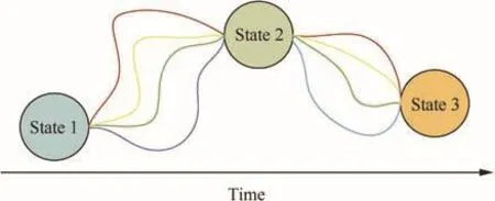
Fig.3 Effects of ROC.

Table 1 Input and output parameters.

Fig.4 Schematic of system.

The pressure coefficient is obtained by the pressure distribution in different positions of the airfoil.The definition of pressure coefficient is illustrated as

The P parameter shows the pressure values acquired by pressure sensors.P∞,ρ∞and V∞show the pressure,density,and flow speed in the free stream,that is in the front of the wind tunnel,respectively.The values are constant for all pressure sensors.These values are measured utilizing a device installed in the front of the wind tunnel.The array of pressure values is converted to a pressure coefficient utilizing Eq.(8).Having pressure coefficients and pressure sensor installation positions,a scalar parameter,S,is defined by

S is called pressure parameter in this study.The input and output parameters of the systems is presented in Table 1.Using the defined inputs and output,a schematic of the system is illustrated in Fig.4.

In this study,the system is an MISO system,which is suitable for the modified LoLiMot algorithm.The datasets are obtained by changing inputs and sampling output of the system.The final locally linearized model of the system is a function like

According to the modified LoLiMot algorithm,the linear function is illustrated as

3.Experimental setup

The system input and output parameters have been described earlier.In order to train the learning algorithm,sets of experiments should be performed to obtain required datasets.The experimental setup of the system is discussed firstly and the experimental scenario is discussed thereafter.The study was carried out on an NACA0012 airfoil.The airfoil is made up of wood so as to minimize electrical conductivity for the best electromagnetic discharge.The airfoil is 45 cm in span and 15 cm in chord.A metal rod connects the airfoil to the setter in a wind tunnel.In the middle of span,23 holes are positioned chord-wise to house pipes for measuring pressure.On the upper surface,the re are 11 holes,and on the lower surface,the re are 12 holes.The positions of the holes are precise and known.Fig.5 illustrates the positions of the pressure holes.

Dielectric barrier discharge actuators are configured in an array of 8 actuators perpendicular to the flow direction.Electrodes and dielectrics are made up of copper and kapton,respectively.Upper electrodes are connected to each other with a high voltage cable.The same is true about lower electrodes.The electrodes are printed on copper and installed on the airfoil with kapton.The design parameters of electric barrier discharge actuators are presented in Table 2.The pressure pipes connected to the pressure holes and the actuators installed on the airfoil are illustrated in Fig.6.

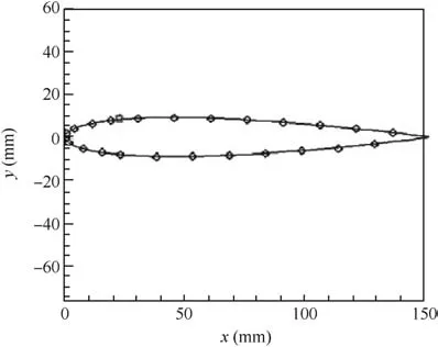
Fig.5 Locations of pressure holes.

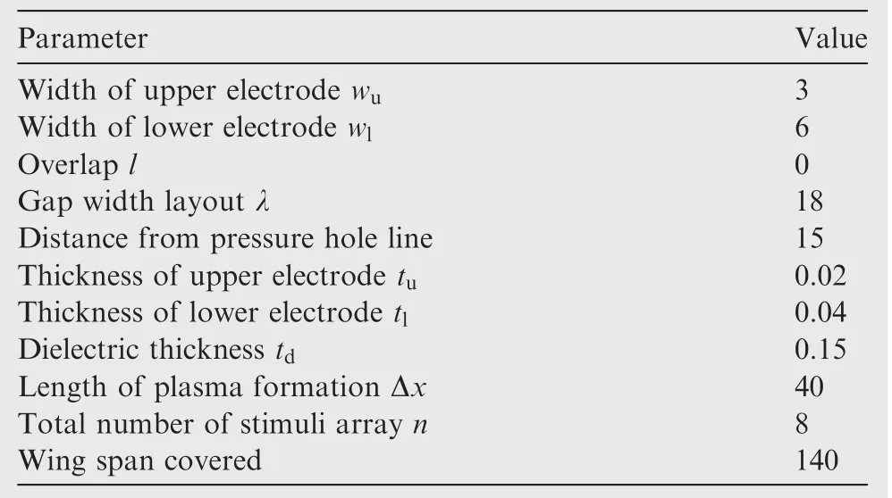
Table 2 Actuator array design parameters expressed in milimeters.

The pipes are connected to pressure sensors in a sensor box.A sensor box is located out of the wind tunnel.In the upper deck of the sensor box,a series of sensors is installed.Each pressure pipe is hooked up to a sensor.The pressure sensors are PX-138005D5V manufactured by OMEGA.The outputs of the sensors are analog.The analog signal wires are connected to an analog-to-digital converter,also called Data Acquisition Card(DAC).The DAC is connected to a computer.The DAC is PCI-1713U manufactured by Advantech.The collection described is responsiblefor acquiring pressure data from the pressure holes located on the airfoil and converting the m to machine data.The sensor box containing sensors,a data acquisition card,and a computer is shown in Fig.7.

All the experiments were performed in the open circuit wind tunnel installed in the Dana Aerodynamic Laboratory at Faculty of Aerospace Engineering,Amirkabir University of Tech.The wind tunnel has a test section of 100 cm×100 cm×180 cm.The wind tunnel fan has a volumetric flow rate of 54 m3/s.The divergence angle in the first diffuser is 3.5°and the diffuser length is 3.5 m.The second diffuser has a divergence angle of 20°,and the disturbances of the tunnel at speeds of 15 m/s and 35 m/s are 0.27%and 0.24%,respectively.The tunnel test room has a divergence angle of 0.5°to prevent the growth of a boundary layer.The floor and ceiling of the tunnel test section also have sheets of Plexiglas plates with a dimension of 34 cm×97 cm and with the possibility of extension that provides access to the model.Because of the smaller size of the airfoil compared to that of the test section and in order to have two-dimensional flow,two Plexiglas screens with a size of 90 cm×100 cm and a thickness of 10 cm on both sides of the airfoil were utilized.As stated by Selig et al16,in order to have two-dimensional flow,the length of Plexiglas sheets should be 6 times longer than the airfoil chord.Fig.8 illustrates the wind tunnel with the airfoil installed inside.

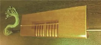
Fig.6 NACA0012 used in experiment.

Fig.7 Sensor box.

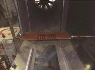
Fig.8 Wind tunnel test section with airfoil installed inside.

The test section has an alpha mechanism which is utilized to set the angle of attack of the airfoil.Besides,the alpha mechanism is utilized as a setter to hold the airfoil in the test section.On the alpha mechanism,the re is a digital indicator for measuring the angle of attack.High-voltage cables are connected to both actuators and a high-voltage amplifier.The amplifier converts a sinusoid wave with a low peak-to-peak voltage to a higher one.The amplification coefficient for the amplifier is 800.It means that at the maximum power,the amplifier converts a 10 V peak-to-peak sinusoid wave to an 8 kV peak-topeak sinusoid voltage.The output wave has approximately 200 W of electrical power.The signal source is created by a function generator which produces a sinusoid wave with a 10 V peak-to-peak voltage.The function generator is manufactured by Hameg and the model of the function generator is HMF2525.The peak-to-peak voltage of the source wave and its frequency are set by setting the function generator using USB connection.The computer in the sensor box reads the pressure data and carries out the calculation.The frequency of excitation,peak-to-peak voltage,flow velocity,and angle of attack are set in each sampling.A schematic of the experimental setup is illustrated in Fig.9.

4.Experiments results

As mentioned earlier,the re are four input parameters and one output to the system.In order to train the learning algorithm,a number of datasets should be acquired.The datasets are in（x，y）combination,which means that in different situations of input parameters,the output parameter is acquired.To have a complete dataset,the inputs should be meshed in a credible region.More data points make the function more accurate,and it takes more time to compute.In each mesh node,an output related to the node is needed.The input array for creating a mesh is illustrated as

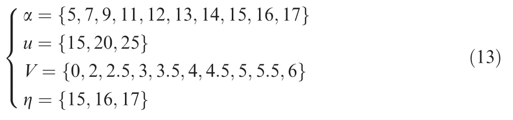
Parameter α,angle of attack,is broken into 10 elements,parameter u,flow velocity,is broken into 3 elements,parameter V is broken into 10 elements,and parameter η,frequency of excitation,is broken into 3 elements.According to the input array,a mesh with 900 nodes is created.For each node,sampling is repeated for 3 times with each time taking 5 s,and the average output data is saved.The saved data for each mesh node is fed to the learning algorithm.Finally,the locally linearized model is created.To evaluate the locally linearized model,a set of experiments was planned.In the experiment,a situation based on the 4 input elements is set,and the experimental value of the S parameter and the calculated value from the model are compared.For the first two of the four parameters,three different states were defined.For the last two parameters,two different states were defined.The definitions are shown as follows:

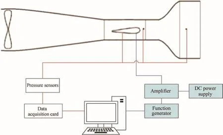
Fig.9 Schematic of experiment setup.

Based on the definitions,36 experiments were planned.For each experiment,the experimental and calculated values of S are compared.Table 3 shows the experiments scenario for validation.

As mentioned earlier,in order to train the learning algorithm,two parameters should be set.The first parameter is the neuron number and the other is the divergence factor.These two parameters affect the error index.To set the se parameters,the error index and neuron number should be compared.The algorithm is trained with the fed data by up to 100 neurons.The training process is repeated with various divergence factors.The divergence factor,γ,is listed as

Fig.10 shows the error index.As illustrated in the figure,an increase in the neuron number causes a decrease in the error index.It means that a higher neuron number makes a more accurate model,but it doesn’t mean that the highest possible number of neurons should be selected.This will be discussed later.From Fig.10,an increase in the divergence factor causes an increase in the error index.This increase is obvious in Fig.10.

The divergence factor controls the fitted function in each of the subspaces.It means how much the fitted function is close to the datasets.A lower divergence factor means that the function should be as close as possible to the datasets.It makes the fitting process harder,because the algorithm should be meticulous in subspace creation.A closer look at Fig.10 reveals that the process is not always constant.For some neuron numbers,the divergence factor doesn’t affect the error index directly but reversely.The error index experiences a reasonable value in more than 80 neurons.The neuron number and divergence factor pairs in which the error index is lower than 0.1 are tabulated in Table 4.The run time for each pair is shown in the table.

Table 3 Experiment scenario for validation.

Fig.10 Error index variation.

As mentioned earlier,an increase in the number of neurons causes a decrease in the error index,so it might be wise to choose the highest number of neurons.When the neuron number reaches a specific amount for each divergence factor,the algorithm cannot fit a locally linearized function in the created subspaces.In this situation,the error index experiences a sudden jump.For a given divergencefactor,the number of neurons in which the divergence occurs is presented in Table 5.

It is noteworthy that changing the fed datasets changes the situation for the algorithm to diverge.To show the divergence of the algorithm,a pair of the neuron number and divergencefactor is chosen.Fig.11 illustrates the divergence of the algorithm for the pair of(292,4).

According to Table 4,the chosen neuron number and divergence factor pair is(90,2).The value is chosen based on the table and figures presented,and nine hundred dataset points were fed to the learning algorithm which is set to have 90 neurons and a divergence factor of 2.In order to be certain about the learning algorithm error,a graph is drawn to show the experimental output and the locally linearized function output.Fig.12 illustrates the comparison between the two types of outputs.For proper illustration,the variance of experimental and model outputs is shown in Fig.13.

According to Fig.13,the maximum error of the algorithm is about 0.09.The error index shows similar values.It guarantees that the learning algorithm has fitted a function correctly.The graph shows that the maximum value of the S parameter is approximately 2.1.To make the error index dimensionless,it should be about 4.2%.This happens when the input data fluctuates,especially while actuators are working to inject momentum.In this occasion,especially when the re is an increase in the peak-to-peak voltage for the input wave of actuators,the output of the system fluctuates.This is important for optimal control of separation utilizing dielectric barrier discharge.

To be certain about the credibility of the locally linearized function representing a model for the system,a series of 36 experiments was carried out.Fig.14 illustrates the experimental and model outputs.

In all the experiments,the model and experimental outputs are close to each other.This certifies the model behavior.In all the experiment,the variance of the model and experimental outputs is negligible.This means that comparing the highest value of S,which is 2.1,the maximum variance is about 1%.The presented model is credible in the entire defined region in which the algorithm is trained.In order to study the graphbetter,Fig.14 is converted into the variance of the two output types,and the variance is dimensionless by the maximum value of S,which is 2.1,and expressed in percentage.The converted graph is shown in Fig.15.

Table 4 Acceptable error indexes.

The variance of the outputs is shown in Fig.15.The maximum variance is just less than one percentage of the maximum value of S.The variance is not constant and sometimes expe-riences jumps.To be certain about the credibility of the locally linearized function,for a constant flow velocity,the output of the model is graphed.In this graph,like other aerodynamic graphs for airfoils,the S parameter should have increased and the n fallen after the separation based on the angle of attack.Fig.16 shows the variation in the S parameter.In the graph,after an angle of attack of 11,the flow experiences a separation and the dielectric barrier discharge tries to avoid the separation.

Table 5 Divergence condition.

Fig.11 Divergence of learning algorithm.

Fig.12 Comparison of outputs.

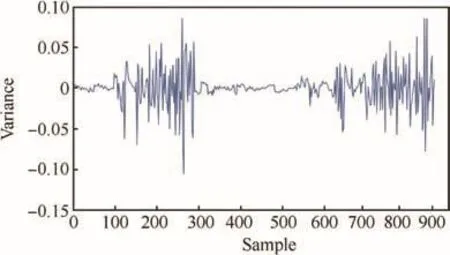
Fig.13 Variance of experimental and model outputs.

Fig.14 Verification experiments.

Fig.15 Converted graph of variance of outputs.

Fig.16 S parameter analysis.

5.Conclusions

To study a system’s behavior,the behavior should be modeled.A model of the system means defining the behavior of the system utilizing a mathematical equation.There are various methods for presenting a model for a system.Several researches have been carried out for developing a method.One of the most common methods is order reduction of governed equations.Using some assumptions and reducing orders of mathematical equations,the governed equation is converted into a simple reduced-order equation which can represent the system.

In this study,a neural network model is utilized in order to neglect governing equations in a system and simplify the modeling procedure.This method converts a complex system of airfoil and DBD to a simple function.

The paper shows the presented model and its validity.Even though the accuracy of the presented model is dependent to the data that is trained in the model,the validation experiment reveals that the final error of the model is negligible compared to experimental results and the presented model is credible enough.Based on the results,the error index doesn’t change significantly while increasing the neuron number to more than 160 neurons.Increasing the neurons number from 160 to 280 causes a 0.03 decrease in the error index and simultaneously increases the processing time.The validation experiment tests the presented model in a random situation in order to verify it.The verification test reveals that the error of the presented model is 1%in the worst case of the test.The average error of the presented method is about 0.15%.The biggest problem of the algorithm is the need of the algorithm to be trained before being used.It takes a lot of time for the algorithm to create the model.These are all valid if the sampling of the system is correct.The sampling procedure should be done in a stable and continuous situation.Besides,the algorithm can be retrained during utilization to make it more accurate.More samples make the results more accurate.It should be noted that in the retrain process,the algorithm uses all the data points to be retrained.

The represented method is credible enough to be relied on in model creation.It is suggested that the game rule should be modified in order to make the accuracy of the algorithm independent from the fed datasets.On the other hand,it is suggested to consider other parameters in the learning algorithm.

Acknowledgements

This study was co-supported by University of Tehran and the Dana Research Laboratory of Amirkabir University of Technology in Iran.

1.Hosain ML,Fdhila RB.Literature review of accelerated CFD simulation methods towards online application.Energy Proc 2015;75:3307–14.

2.Nelles O.Nonlinear system identification:from classical approaches to neural networks and fuzzy models.Appl Ther 2001;6(7):717–21.

3.Barbagallo A,Sipp D,Schmid PJ.Input-output measures for model reduction and closed-loop control:application to global,modes.J Fluid Mech 2011;685:23–53.

4.Pinier JT,Ausseur JM,Glauser MN,Higuchi H.Proportional closed-loop feedback control of flow separation.AIAA J 2007;45(1):181–90.

5.Dandois JE,Garnier P,Pamart Y.NARX modelling of unsteady separation control.Exp Fluids 2013;54(2):1–14.

6.Gad-el-hak M.Flow control:passive,active and reactive flow management.1st ed.Cambridge:Cambridge University Press;1999.

7.Cattafesta LN,Sheplak M.Actuators for active flow control.Ann Rev Fluid Mech 2011;43(43):247–72.

8.Yang LL,Li J,Cai J,Wang G,Zhang Z.Lift augmentation based on lf ap deflection with dielectric barrier discharge plasma flow control over multi-element airfoils.J Fluids Eng 2016;138(3):031401.

9.Cho YC,Wei S.Adaptive flow control of low-Reynolds number aerodynamics using dielectric barrier discharge actuator.Prog Aerosp Sci 2011;47(7):495–521.

10.Mohammadreza G,Kazimierz A,Castle GSP.Quasi-stationary numerical model of the dielectric barrier discharge.J Electrostat 2014;72(4):261–9.

11.Sjo¨berg M,Serdyuk YV,Gubanski SM,Leijon MA˚S.Experimental study and numerical modelling of a dielectric barrier discharge in hybrid air–dielectric insulation.J Electrostat 2003;59(2):87–113.

12.Tian Y,Cattafesta L,Mittal R.Adaptive control of separated flow.Reston:AIAA;2006.Report No.:AIAA-2006–1401.

13.Kalhor A,Araabi BN,Lucas C.Reducing the number of local linear models in neuro-fuzzy modeling:a split-and-merge clustering approach.Appl Soft Comput 2011;11(8):5582–9.

14.Kalhor A,Araabi BN,Lucas C.An online predictor model as adaptive habitually linear and transiently nonlinear model.Evolving Syst 2010;1(1):29–41.

15.Anderson JD.Modern compressible flow:with historical perspective.Boston:McGraw-Hill;2003.

16.Selig MS,Guglielmo JJ,Broern AP,Giguere P.Experiments on airfoils at low Reynolds numbers.Reston:AIAA;1996.Report No.:AIAA-1996–0062.

4 August 2016;revised 26 September 2016;accepted 28 October 2016 Available online 24 August 2017

Dielectric barrier discharge;

Flow separation;

Mathe matical model;

NACA0012 airfoil;

Neuro-fuzzy

*Corresponding author.

E-mail address:kosari_a@ut.ac.ir(A.KOSARI).

Peer review under responsibility of Editorial Committee of CJA.

Production and hosting by Elsevier

http://dx.doi.org/10.1016/j.cja.2017.08.007

1000-9361©2017 Production and hosting by Elsevier Ltd.on behalf of Chinese Society of Aeronautics and Astronautics.This is an open access article under the CC BY-NC-ND license(http://creativecommons.org/licenses/by-nc-nd/4.0/).

©2017 Production and hosting by Elsevier Ltd.on behalf of Chinese Society of Aeronautics and Astronautics.This is an open access article under the CC BY-NC-ND license(http://creativecommons.org/licenses/by-nc-nd/4.0/).