Two-Dimensional Direction Finding via Sequential Sparse Representations

Yougen Xu, Ying Lu, Yulin Huang and Zhiwen Liu(School of Information and Electronics, Beijing Institute of Technology, Beijing 100081, China)

Two-dimensional (2D) direction finding has found wide application in practical systems like radar, sonar, wireless communications, medical imaging, and space science. Representative 2D direction finding methods include 2D multiple signal classification (MUSIC), 2D estimation of parameters via rotational invariance technique (ESPRIT), and 2D maximum likelihood[1-2].

Recently, the sparse representation technique has been developed for one-dimensional (1D) narrowband or wideband direction finding, in the element, covariance, or subspace domains[3-11].However, the computational burden of the sparse representation scheme may be prohibitively large when directly adopted for 2D direction finding in a joint processing mode.

To tackle this problem, the decoupled sparse representation strategy has been proposed for computationally acceptable 2D direction finding[12].An alternative way for the reduction of computational complexity is to apply two separate sparse representation procedures to some specific array structures, for example, the parallel or separate sparse representation techniqueusing an L-shaped array[13]. However, an extra pairing step is required by this method due to its separate processing nature.

In this paper, a pairing free sequential sparse representation method is proposed for 2D direction finding by using a multi-layer L-shaped array. To make exact sparse representations, the weighted smoothing techniques for the L-shaped array are taken into account, for the respective estimation of the elevation angles and the azimuth angles.The second order statistics of the two vectors for sparse representation are also derived, which can be used for the determination of the regularization parameters needed for sparse restoral.

Throughout the paper, “E” denotes expectation, “(·)T”, “(·)H”, and “(·)*” denote transpose, conjugate transpose, and conjugate; “Re (·)” and “Im (·)”signify the real part and imaginary part; ‖·‖1and ‖·‖2represent the l1norm and l2norm; “⊗”, “⊙”, and “∘” denote the Kronecker product, Hadamard product, and tensor outer product, respectively.“IN” and“1”denote theN×Nidentity matrix and all-one vector, “vec (·)”is the vectorization operation, and “tr (·)”is the trace of a matrix.

1 Problem Formulation

Consider an array composed ofN1L-shaped sub-arrays along thez-axis, each of which hasN2=Nx+Ny-1 sensors, withNxalong thexleg andNyalong theyleg, respectively, as shown in Fig.1. The sensors are omnidirectional and the normalized inter-element spacing in signal wavelength isd.

Fig.1 Structure of the array

WithMfar-field narrowband signals incident on the array, the array output tensor can be written as

(1)

(2)

(3)

and N(t)=[n1(t),n2(t),…,nN1(t)]T, in which nn(t) is the noise vector of then-th sub-array. Here the noise is assumed to be spatially white with powerσ2and independent of the incident signals.

The array output covariance tensor is given by

(4)

In practice, T can be estimated as follows.

(5)

whereKis the snapshot number.

2 Proposed 2D Direction Finding Method

2.1 Estimation of elevation angles

From Eq.(4) we can get

(6)

(7)

where S=E{s(t)sH(t)}, s(t)=(s1(t),s2(t),…,sM(t))T,

(8)

It follows that

(9)

(10)

whereσ(z)=(1Tw(z))σ2, and w(z)is anN2×1 non-zeroreal-valued weight vector.

In order to apply sparse representation, w(z)is such selected that S(z)is a diagonal matrix with non-zero diagonal entries. To this end, we note from Eq.(2) and Eq.(7) that R(z)would be a Toeplitz matrix if S(z)is perfectly diagonalized. Hence, w(z)can be obtained by solving the following problem[14]:

(11)

where

(12)

in which

(13)

and, forq=1,2,…,N2,

(14)

The solution to Eq.(11) can be obtained by using the Lagrange method, as

(15)

If S(z)is perfectly diagonalized, we have that

(16)

(17)

where

(18)

(19)

(20)

(21)

where

(22)

From Eq.(21), the estimation of the elevation angles can be reduced to the localization of the non-zero elements of t(z)which, given w(z), can be obtained by solving the following problem with the convex optimization toolbox (CVX[15]):

(23)

whereα(z)is the fitting error threshold, and

(24)

Recall that the signals are assumed to be circularly symmetric, and X(tk1) is independent of X(tk2) fork1≠k2; therefore, it can be derived that, given w(z),

(25)

Then,α(z)can be determined as

(26)

whereβ(z)is a pre-specified weight factor.

2.2 Eestimation of azimuth angles

From Eq.(4) we can get

(27)

where

(28)

(29)

It follows that

(30)

(31)

whereσ(xy)=(1Tw(xy))σ2, and w(xy)is anN1×1 non-zero real-valued weight vector.

It can be verified from Eq.(3) and Eq.(28) that R(xy)would be a block-Toeplitz matrix given that S(xy)is completely diagonalized, based on which w(xy)can be determined by using the method given in Ref.[16].

Here, an alternative method is proposed based on the direct diagonalization of S(xy), making use of the estimates of elevation angles obtained in Section 2.1.

First, from Eq.(31) we have that

S(xy)(m,k)=[(w(xy))Tbm,k]S(m,k)

(32)

Furthermore, S(xy)is a Hermitian matrix,consequently, to make S(xy)a diagonal matrix, it is required that S(xy)(m,k)=0, or more precisely,

[w(xy)]TRe(bm,k)=0,
2≤m≤M,1≤k≤M-1,m>k

(33)

[w(xy)]TIm (bm,k)=0, 2≤m≤M,1≤k≤M-1,m>k

(34)

As a result, w(xy)can be determined by solving the following problem as

(35)

where

(36)

(37)

(38)

If S(xy)is perfectly diagonalized, we have

(39)

It then follows from Eq.(30) that

(40)

where

(41)

(42)

(43)

From Eq.(40), 2D direction finding can be realized by a direct 2D sparse representation of v(xy). This however is computationally too expensive[10]. We now present a more efficient method by using the elevation angle estimates obtained in the Section 2.1.

(44)

where

(45)

(46)

whereα(xy)is the fitting error threshold, and

(47)

(48)

Then,α(xy)can be determined as

(49)

whereβ(xy)is a pre-specified weight factor.

Again, the problem Eq.(46) can be solved by using the CVX toolbox.

We point out finally that the decoupled and parallel sparse representation schemes apply also to R(xy)by noting that

(50)

where cos ϑm=cosθmsinφm, cosφm=sinθmsinφm.

We will compare the proposed sequential method with the 2D, decoupled, and parallel methods in terms of 2D direction finding accuracy and computation efficiency in the following simulation section.

3 Simulation Results

The structure setting of the array used in the simulations isN1=6,Nx=5,Ny=6, andd=0.5.

In the first example, we consider two uncorrelated signals from (40.6°,30.5°) and (-27.8°,50.3°), respectively. The signal-to-noise ratio (SNR) is 0 dB, and the number of snapshots is 500. The two weight factors,β(z)andβ(xy), defined in Eq.(26) and Eq.(49), respectively, are equal to one. The elevation spectrum and azimuth spectrum are shown in Fig.2 and Fig.3, respectively. It is seen from the figures that the two signals are clearly resolved.

Fig.2 Elevation spectrum (for two uncorrelated signals, the SNR value is 0 dB, and the number of snapshots is 500)

In the second example, we consider two coherent signals from (40.6°,30.5°) and (-27.8°,50.3°), respectively. The SNR value is 0 dB, and the number of snapshots is 500,β(z)=1, andβ(xy)=1. The elevation spectrum and azimuth spectrum are shown in Fig.4 and Fig.5, respectively. Satisfactory 2D direction finding performance of the presented method is observed again.

Fig.3 Azimuth spectrum (for two uncorrelated signals, the SNR value is 0 dB, and the number of snapshots is 500)

Fig.4 Elevation spectrum (for two coherent signals, the SNR value is 0 dB, and the number of snapshots is 500)

Fig.5 Azimuth spectrum (for two coherent signals, the SNR value is 0 dB, and the number of snapshots is 500)

In the third example, we compare the performances of the presented method (sequential SR) with the 2D, decoupled, and parallel sparse representation schemes (referred to as 2D SR, decoupled SR, and parallel SR, respectively),in terms of 2D direction finding accuracy and computational complexity. Two uncorrelated signals from (-20°,30°) and (45°,60°) are considered, andβ(z)=1,β(xy)=1. The regularization parameters used by the 2D, parallel, and decoupled sparse restoral are all selected as 1.

The experimental root mean square error (RMSE) curves of the compared methods versus the SNR values (0 dB) and the number of snapshots (500) are displayed in Fig.6 and Fig.7, respectively.The computation efficiency comparison of the methods are given in Tab.1.

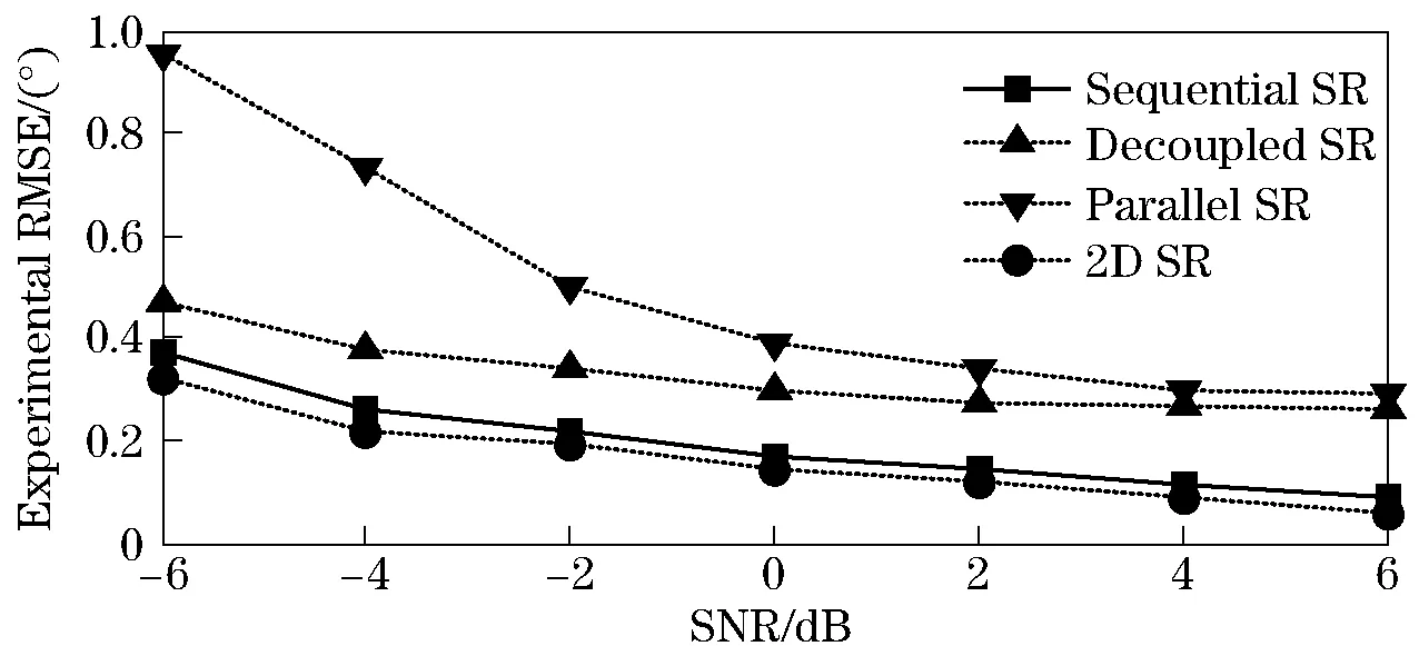
Fig.6 Experimental RMSE curves of the compared methods against the SNR values

Fig.7 Experimental RMSE curves against the number of snapshots

Tab.1 Computation efficiency comparison of the methods

It is observed from the results that, under the tested scenario and with the aforementioned regularization parameter selection, the proposed sequential SR method outperforms the decoupled SR method in both 2D direction finding performance and computational complexity. While having the least computational burden, the parallel SR method is inferior to the other three methods in direction finding precision. The 2D SR method performs the best while having the heaviest computational burden.

In summary, a good trade-off between 2D direction finding accuracy and computation efficiency has been observed for the proposed sequential SR method.

4 Conclusion

A sequential sparse representation based method for 2D direction finding has been proposed. The sizes of the dictionary matrices constructed in the sparse representations for estimating the elevation angles and azimuth angles are of the same order as the 1D sparse representation schemes. The performance of the sequential method has been demonstratedby simulation results. The comparisons of the sequential method with the 2D, decoupled, and parallel methodshave also been given.

[1] Chan A Y J, Litva J. MUSIC and maximum likelihood techniques on two-dimensional DOA estimation with uniform circular array [J].IEEE Proceedings Radar, Sonar and Navigation,1995, 142(3):105-114.

[2] Li J, Compton R T.Two-dimensional angle and polarization estimation using the ESPRIT algorithm [J]. IEEE Transactions on Antennas and Propagation,1992, 40(5):550-555.

[3] Fuchs J J. On the application of the global matched filter to DOA estimation with uniform circular arrays [J]. IEEE Transactions on Signal Processing, 2001, 49(4): 702-709.

[4] Malioutov D, Cetin M, Willsky A.A sparse signal reconstruction perspective for source location with sensor arrays [J]. IEEE Transactions on Signal Processing, 2005, 53(8):3010-3022.

[5] Hyder M M, Mahata K. Direction-of-arrival estimation using a mixedl2,0norm approximation [J]. IEEE Transactions on Signal Processing, 2010, 58(9): 4646-4655.

[6] Liu Z M, Huang Z T, Zhou Y Y. Direction-of-arrival estimation of wideband signals via covariance matrix sparse representation [J]. IEEE Transactions on Signal Processing, 2011, 59(9): 4256-4270.

[7] Yin J H, Chen T Q. Direction-of-arrival estimation using a sparse representation of array covariance vectors[J]. IEEE Transactions on Signal Processing, 2011, 59(9):4489-4493.

[8] He Z Q, Shi Z P, Huang L, et al. Underdetermined DOA estimation for wideband signals using robust sparse covariance fitting [J]. IEEE Signal Processing Letters, 2015, 22(4): 435-439.

[9] Hu N, Ye Z F, Xu D Y, et al.A sparse recovery algorithm for DOA estimation using weighted subspace fitting [J]. Signal Processing, 2012, 92(10):2566-2570.

[10] He Z Q, Liu Q H, Jin L N, et al.Low complexity method for DOA estimation using array covariance matrix sparse representation [J]. Electronics letters, 2013, 49(3): 228-230.

[11] Shen Q, Liu W, Cui W, et al. Low-complexity direction-of-arrival estimation based on wideband co-prime arrays [J]. IEEE/ACM Transactions on Audio, Speech, and Language Processing, 2015, 23(9): 1445-1456.

[12] Luo X Y, Fei X C, Wei P, et al. Sparse representation-based method for two-dimensional direction-of-arrival estimation with L-shaped array [C]∥IEEE International Conference on Communication Problem-Solving, Beijing, China, 2014.

[13] Li Pengfei, Zhang Min, Zhong Zifa.Two dimensional DOA estimation based on sparse representation of space angle [J]. Journal of Electronics and Information Technology, 2011, 33(10):2402-2406. (in Chinese)

[14] Takao K, Kikuma N.An adaptive array utilizing an adaptive spatial averaging technique for multipath environments [J]. IEEE Transactions on Antennas and Propagation, 1987, 35(12):1389-1396.

[15] Grant M, Boyd S.CVX: MATLAB software for disciplined convex programming [EB/OL]. (2010-04-01). http:∥cvxr.com/cvx.

[16] Xu Y G, Liu Z W.Polarimetric angular smoothing algorithm for an electromagnetic vector-sensor array [J]. IET Radar, Sonar and Navigation,2007, 1(3):230-240.