Electromagnetism-Like Mechanism Algorithm with New Charge Formula for Optimization

YIN Feng(印 峰)， KANG Yongliang(康永亮)， ZHANG Dongbo(张东波)， QIU Jie(邱 杰)

1 College of Automation and Electronic Information， Xiangtan University， Xiangtan 411105， China

2 National Engineering Laboratory of Robot Vision Perception and Control Technology， Xiangtan University， Xiangtan 411105， China

Abstract: The electromagnetism-like (EM) algorithm is a meta-heuristic optimization algorithm，which uses a novel searching mechanism called attraction-repulsion between charged particles. It is worth pointing out that there are two potential problems in the calculation of particle charge by the original EM algorithm. One of the problems is that the information utilization rate of the population is not high， and the other problem is the decline of population diversity when the population size is much greater than the dimension of the problem. In contrast， it is more fully to exploit the useful search information based on the proposed new quadratic formula for charge calculation in this paper. Furthermore， the population size was introduced as a new multiplier term to improve the population diversity. In the end， numerical experiments were used to verify the performance of the proposed method， including a comparison with the original EM algorithm and other well-known methods such as artificial bee colony (ABC)， and particle swarm optimization (PSO). The results showed the effectiveness of the proposed algorithm.

Key words: electromagnetism-like (EM) mechanism； stochastic search method； constrained optimization； global optimization； attraction-repulsion

Introduction

The problem that is addressed in this paper considers finding a global optimal solution to a nonlinear constrain optimization problem：

minf(x)，

s.t.gi(x)≤0，i=1， 2， …，m，

hj(x)=0，j=m+1，m+2， …，m+p，

x∈Ω，

(1)

where，f，gandhare nonlinear continuous functions； the closed setΩis defined byΩ={x∈Rn：l≤x≤u}；mandprepresent the number of inequality constraints and equality constraints， respectively. The stochastic-type algorithm， such as electromagnetism-like (EM) algorithm， is one of the most important solving methods for problem formula(1). The key idea of the EM algorithm is to treat all searching particles as electrical charges and simulate the attraction-repulsion principle in electromagnetism theory in order to move particles towards the position of the optimal solution[1-2]. In the past decade， there were many improved versions of the original EM algorithm. For example， some articles optimized the initial population to make it more evenly distributed in the feasible region. Jiangetal.[3]used the good point set principle in number theory to construct the initial population. The uniform design method was also applied to the initial population[4-5]. Some articles modified the charge formula. A new scaling factor was introduced into the formula for point charge[6]， and this scaling factor was relative to the difference between the best and the worst function values in the population. Furthermore， some other articles optimized the local search strategies. The pattern search method of Hooke and Jeeves was used for local search[7]. Researchers[8-9]used tabu search or genetic algorithm instead of the random search. Rocha and Fernandes[10]also modified the total force formula and the move operator， and the effect of obtained forces in previous iterations was considered when calculating the total force exerted on points at the current iteration. Tsengetal.[11]developed a novel attraction-repulsion operator to move particles in the population. Meanwhile， the idea of combinatorial optimization is also widely used to improve the performance of the EM algorithm. The common hybrid methods include the combination of Genetic， Solis and Wets， modified Davidon-Fletcher-Powell (DFP) and particle swarm optimization (PSO)[12-15]. To resolve a discrete optimization problem， the EM algorithm was combined with Firefly algorithm[16]. An efficient hybrid method combined EM and chaos searching technique was presented to solve the nonlinear bilevel programming problem[17]. Inspired by the collective animal behavior， a new algorithm called collective EM optimization (CEMO) can efficiently register and maintain all possible optimal solutions[18]. Tanetal.[19]proposed an experiential learning EM algorithm (ELEM)， which was integrated with two new components of particle memory， experience analyzing and decision. Researchers[20-21]utilized the opposition-based learning (OBL) approach to improve convergence speed. Miao and Jiang[22]proposed a linear classification method based on an improved EM algorithm. Jiangetal.[23]designed an EM algorithm suitable for classification to solve support vector machine (SVM) decision-tree multi-classification strategy. Moreover， researchers[24-26]applied improved EM algorithms to various types of incident vehicle routing problem (IVRP).

Although the original EM has powerful capabilities， it cannot be used directly to solve optimization problems with constrains like problem (1). Many modified versions are proposed to solve this problem. One common approach is to convert problem (1) into an unconstrained problem via a penalty function[27]. However， the inherent difficulty is the choice of the penalty parameter in the penalty function-based methods. Other effective method is the use of the feasibility and dominance (FAD) rules for the constraints handling in constrained global optimization[28]. These rules can be easily incorporated into the EM algorithm. Based on this， the EM algorithm can directly handle the constrained optimization problem without any changes. By introducing a new formula of charge calculation based on both the function value and the total constraint violations， the performance of the above hybrid EM algorithm combined with FAD rules can be improved further[29].

In this paper， a modified EM algorithm with a new formula for charge calculation is proposed. Compared to the original formula， the magnitude of charge is proportional to the absolute value of the objective function according to the new formula. Its greatest advantage is that it can make full use of the heuristic information of more particles. Moreover， we multiply the fraction by the size of populationminstead of dimensionnto void over-concentration of charges， which helps to improve the diversity of population. Finally， the rules of FAD are added to the proposed modified algorithm in order to apply the EM algorithm to solve constrained optimization problem.

1 Analysis of EM Algorithm

1.1 Brief reviews of EM algorithm

The EM algorithm is a stochastic search method for global optimization. The complete process consists of four steps： initialization， local search， calculation of charge and total force vectors， and movement of points. As a simple example， Fig. 1 is used to illustrate the search mechanism of the EM algorithm. Assume that the current particle to be moved is particle 3， and the function values corresponding to the positions of the three particles are 5， 10， and 15， respectively. For a minimization optimization problem， particle 3 is better than particle 1 while worse than particle 2. According to attraction-repulsion mechanism of the EM algorithm， particle 3 is repulsed by particle 1 and attracted by particle 2. As a result， particle 3 searches in the direction of the resultant vectorF. More details about the EM algorithm are available in Ref.[1].

Fig. 1 An illustration of attraction-repulsion force

1.2 Drawbacks of original EM algorithm

First of all， it needs to be pointed out that we only consider the effect of charge. As mentioned earlier， all points in the EM algorithm are seen to be charged particles whose values are determined by the following formula：

(2)

where，f(xi) andf(xbest) represent the objective function value for the pointiand the current best point， respectively， and the point that has the minimum function value is stored inxbest；nis the dimension of problem；mis the size of population. According to Eq. (2)， the values of charges range in[0， 1]. The points that have smaller objective function values will possess higher charges， as shown in Fig. 2. Particularly， the best particles will have a maximum charge of 1.0. For the EM algorithm， the charges will determine the force magnitude. The higher values of charges are， the higher the magnitude of attraction is. Contrarily， the points with worse objective function value produce a weak repulsive force. Then， the points in the population will move towards the region around the better points. However， Eq. (2) has two potential problems.

(1) Population diversity. This issue usually occurs whenmis much greater thann. With the increase ofm， the values of the exponential term will obviously tend to zero in Eq. (2). As a result， all values of charges will be clustered around 1.0 (illustrated by the line 2 in Fig. 2). At this time， there is no obvious difference between the “good point” and the “bad point”. This process is termed as “population diversity lost”. Remember that better points should possess higher charges. Then it is not conducive to the exploration of the solution to the problem when the population diversity is lost.

(2) Search information utilization. According to Eq. (2)， we can see that worse points will possess lower charges. In particular， the worst point in the population has the lowest charge. As a result， the force produced by these particles with small charges may be too small to be ignored. In other words， the role of these points will be weakened in searching， especially for those have near-zero charges (illustrated by line 1 in Fig. 2). Obliviously， if the charge of a particle is 0， this particle will not play any role in the search process. This process is termed as “search information lost”.

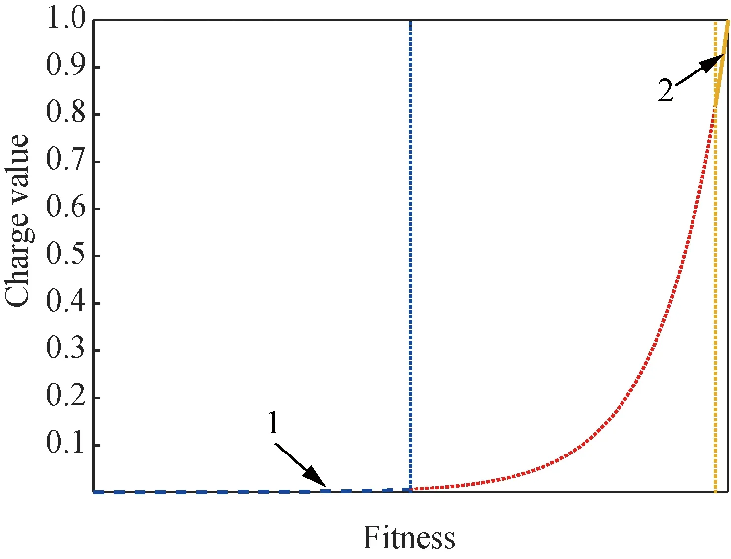
Fig. 2 Typical distribution of charge values calculated by Eq. (2)

1.3 New formula of charge

To improve the performance of the EM algorithm， we construct a new formula to replace Eq. (2) to calculate charges：

(3)

Equation (3) makes use of the monotonicity of the quadratic function， which can ensure that the charges of worse particles are not 0 or close to 0. The coefficients 4 and 0.5 in Eq. (3) are combined to make the curve cross pass through points (0， 1) and (1， 1)， so as to ensure the charge distribution in[0， 1]. Moreover， the total number of particlemis introduced to replacenin Eq. (2).When we select a larger number of particlem， in general， the following inequality relation holds：

(4)

Thus， by multiplying the termm， we can effectively avoid the situation that the charge distribution is too concentrated when the ratio of the fraction in Eq. (3) tends to 0. A typical distribution of charges obtained by Eq. (3) is shown in Fig. 3.

Fig. 3 Typical distributions of charge values by using new Eq. (3)

As can be seen from Fig. 3， the charges of most particles are far from 0 compared with those in Fig. 2. Moreover， even a worse particle like pointain Fig. 3 can be assigned a higher amount of charge based on the new formula. Compared to the original algorithm， the modified formula can make better use of heuristic information contained in “bad points”. To illustrate the difference between the two formulae， let us consider a simple case. There are three particles on a straight line， as shown in Fig. 4. Suppose that particle 1 and particle 2 are worse than particle 3 while particle 2 is better than particle 1. Then particle 3 is repelled by repulsion forces from particle 1 and particle 2 respectively. According to Eq. (2)，F23is greater thanF13.As a result，Fis directed to particle 1 and encourages particle 3 to move towards the neighborhood region of particle 1. Obviously， the direction ofFis not optimal as point 1 is worse than point 2. In contrast， a better search direction pointing to the region where particle 2 is located can be obtained by using Eq. (3)， as shown in Fig. 5.

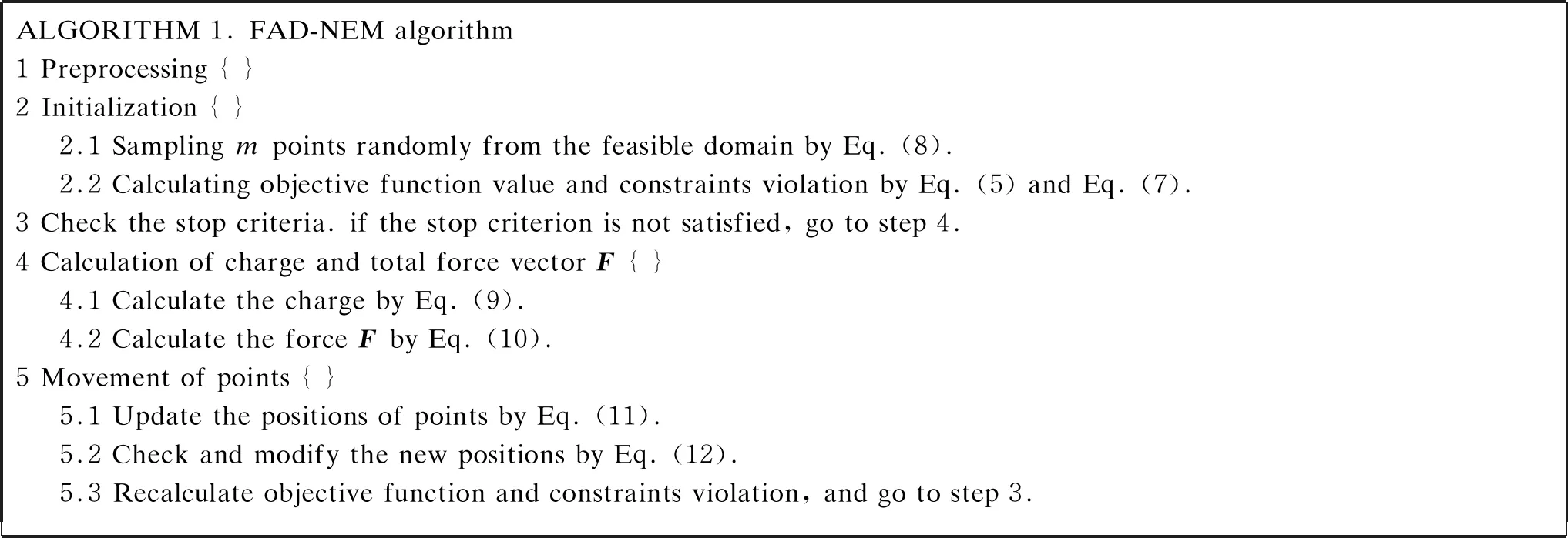
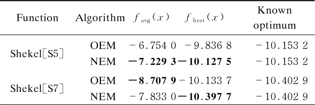
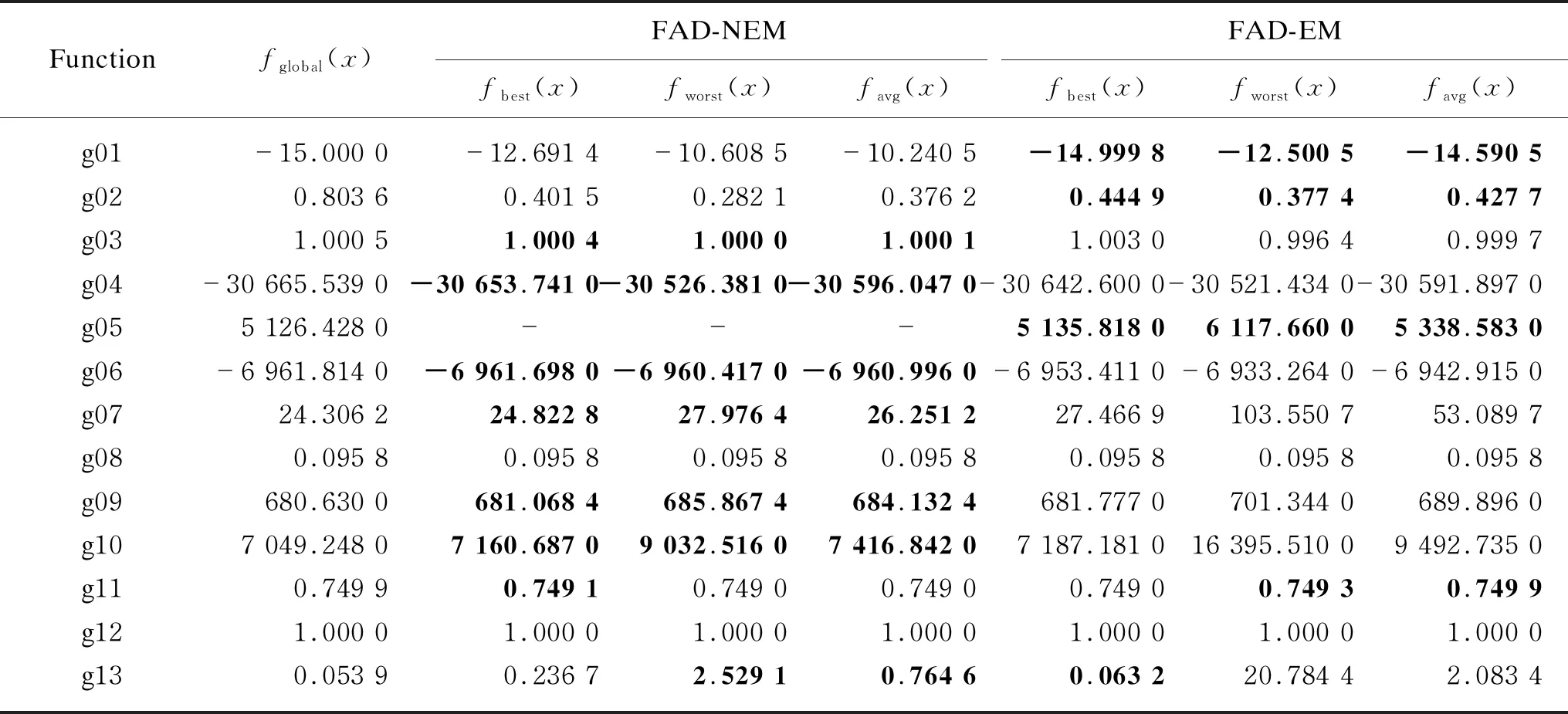
Fig. 4 Non-optimal direction of F pointing to worse solution[q1

Fig. 5 Optimal direction of F pointing to better solution[q1> q2 obtained by using Eq. (3)]

Fig. 6 Scheme of FAD-NEM algorithm

Note that some scholars also improved the charge formula of EM algorithms. Han’s improvement focused on adapting the new charge formula to solve the bi-objective optimization problems[30]， which expanded the application range of EM algorithms. But we are aiming at the improvement of particle’ charge of different fitness， which can make better use of the search information of worse points. A complete description about the revised EM algorithm can be available in section 2.

2 Revised EM Algorithm

In order to solve the constrained optimization problem， a pre-treatment process is involved. The revised EM algorithm consists of five steps： pretreatment， initialization， local search, calculation of charge and total force vectors， and movement of points. Here, the step of local search is omitted.

2.1 Pretreatment

Firstly， the problem (1) is rewritten as

minf(x)，

s.t.c(x)≤0，

x∈Ω.

(5)

In Eq. (5)， all equality constraints in problem (1) have been transformed into inequality forms.

c(x)=(g1(x)，g2(x)， …，gm1(x)， |h1(x)|-ε，

|h2(x)|-ε， …， |hl(x)|-ε)，

(6)

whereεis a constant with a very small value， and constraint violation can be measured by using norm of a vector ‖π(x)‖2.

πj(x)=max{0，cj(x)}，j=1， 2， …，m1+l.

(7)

According to Eq. (6) and Eq. (7)， it can be known that the point is feasible if ‖π(x)‖2=0， otherwise， it is an infeasible point. Then， the fitness of the point can be defined as follows[28].

(1) Compared with infeasible points， the feasible point is better.

(2) Between two infeasible points， the one having lower constraint violation is better.

(3) For two feasible points， the one having lower function value is better.

2.2 Initialization

(8)

Then calculate the objective functionf(xi) of all particles. Compared to the original algorithm， the constraints violation ‖π(xi)‖2is required to be computed for each point in the population additionally. The pair of information (f(xi)，‖π(xi)‖2) defines the fitness of points. The local search process is used to improve the local search performance of the EM algorithm， but it is not necessary.

2.3 Calculation of charge and total force vector

In the EM algorithm， the charge of the particles is relative to their objective function values. In this paper， Eq. (9) is used to calculate the charge. In this way， the points that have high absolute objective value and lower constraints violation possess higher charges. It is noted that it is not necessarily the best one for the point with better objective value in solving constrained optimization problems.

(9)

The charge of each pointi， denoted byqi， determines the power of attraction or repulsion. The total forceFiexerted on pointiis computed by

(10)

According to Eq. (10)， the force between two particles is decided by their fitness. The particle with a better fitness will exert an attraction on another particle.

2.4 Movement of points

After evaluating the total force vectorF， the particleiwill move along the force direction， and the new position is determined by

(11)

whereλis a random step length， andλis assumed to be uniformly distributed between 0 and 1. Note that the new positions should be checked (and modified if necessary) to ensure the allowed feasible movement towards the upper bounduj， or the lower boundlj：

(12)

wherejdenotes thejth element of vectors in Eq. (12). Finally， after updating all particles， the termination criteria will be checked to stop the calculation or repeat the search process. Figure 6 gives the general scheme of the proposed algorithm which uses the feasibility and dominance rules in the new EM mechanism (FAD-NEM) algorithm.

3 Numerical Results

In order to test the performance of the proposed algorithm， some different types of test functions will be used in experiments[31]. For the sake of fairness， the average results for test functions are compared with the average number of evaluations over 25 runs. All computations are conducted on an Intel(R) Core(TM) i5-7200M CPU @2.50GHz Pc. The algorithm is coded in Matlab R2016a.

3.1 Solving un-constrained problems

We will do performance tests on the EM algorithm with different charge formulas in solving un-constrained problems. The selected EM algorithm here is the original version presented by Birbiletal.[1](denoted by OEM)， which uses Eq. (2) to calculate the charges. It is also the most widely used formula in various versions of EM algorithms. As a comparison， we proposed a modified EM algorithm termed as NEM algorithm that directly replaces the original charge formula with Eq. (3). In order to demonstrate the influence of the charge formula more objectively， we apply the EM algorithm without local research procedure. The same test set and parameters as those in Refs.[1， 27]. The test set consists of 15 general test functions and 9 harder test functions. All of them are un-constrained.

As can be seen from Table 1， both OEM and NEM algorithms can successfully find the optimal solutions for Complex， Epistacity， Kearfott， and Sine Envelope functions. But for Davis， Griewank， Himmelblau， Kearfott， Step， and Trid(5) functions， the average solutionfavg(x) and best solutionfbest(x) of the NEM algorithm are better than those of the OEM algorithm.

Table 1 Test results for general test functions

It is noted that the solutions of OEM and NEM for Davis and Trid(20) functions are both less satisfactory than those for other functions. This is mainly due to the fact that the number of evaluations in test is not large enough to adequately explore the feasible space for high-dimension or irregular function[1]. Nevertheless， our results show that the accuracy of solutions is improved by using NEM.

To make a more intuitive comparison， a set of convergence curves are shown in Fig. 7. It can be seen that the NEM has a faster convergence speed in the early stage of the process， and has a better chance to find the optimum solution in the later stage.

Fig. 7 Convergence curve comparison for Trid(5) function

Table 2 shows the results for harder test functions. It can be seen that the test results of both algorithms are satisfactory except for Shekel and Shubert functions. Obviously， the average solutions are all not good for OEM and NEM. The good news is that the best solutions are close to the global optimum by using NEM. It shows that the ability to explore the best solution has been improved by the new charge formula.

Table 2 Test results for harder test functions

(Table 2 continued)

In Table 3， we take the Davis function as an example to analyze the influence of parameters (population sizemand number of iterationsMAXITER). WhenmandMAXITERincrease， the solving accuracy of the two algorithms gradually improves. It is worth noting that there is a similar conclusion for different parameter combinations (mandMAXITER)， excluding a few exceptions that the average solution， the optimal solution， and the standard deviation (Std) of NEM are better than those of OEM. It can be seen from the above experimental results that the performance of the proposed NEM is better than OEM， and is not disturbed by parameters.

Table 3 Performance comparison of OEM and NEM for Davis function

3.2 Solving constrained problems

In this case， we introduce an algorithm that uses FAD-EM algorithm. The FAD-EM algorithm developed by Rocha and Fernandes[28]was compared with ours FAD-NEM algorithm since the same feasibility and dominance rules were used in both algorithms. The comparison of parameters used in ours and the FAD-EM algorithm are as follows： population size (10vs.50)， max-iteration (10 000vs. 350 000)， local search applied (current best pointvs. all points) and local search number (one-time-onlyvs. search coordinate by coordinate). The detailed descriptions of the test functions used are available in Ref.[28].

The results in Table 4 show that the performance of our method is the same as or better than that of the FAD-EM， except for g01， g02 and g05 functions. Among them， the results of two methods are very similar and all exact solutions are found for g03， g08， g11 and g12 functions. For g04， g06， g07， g09， g10 and g13 functions， the test results of ours are better than those of algorithms in Ref.[28]. Our results also show that the inherent defects of the EM algorithm make it impossible to find the optimal solution for this kind of problem including too many constraints or variables. For example， for high-dimension or irregular problems， such as g01， g02 and g05 functions， neither method can get the feasible solutions. Both two methods are able to approximate the optimum in most of the problems. Note that our method uses more stringent conditions in the test. From this point of view， the proposed algorithm shows better performance in exploring better solutions.

Table 4 Comparisons of FAD-NEM with FAD-EM

Furtherly， more comparative experiments are carried out. The heuristic methods to be compared include PSO， particle evolutionary swarm optimization (PESO)， Toscano and Coello’s PSO (TCPSO)， stochastic ranking (SR)， differential evolution (DE) and artificial bee colony (ABC). The test functions and results of the compared methods are available in Ref.[28]. FAD-EM and the other algorithms mentioned above test the given function， and the statistical results show that better， equal， and worse indicators are 5.12%， 29.49%， and 65.39%, respectively[28]. In contrast， the test results for the proposed method FAD-NEM are 7.69%， 47.44%， and 44.87% respectively. The proportions of better and equal results are improved by using the proposed algorithm in this paper.

4 Conclusions

This paper proposed an improved EM algorithm with new charge calculation formulas. It can not only improve the utilization of search information， but also improve the diversity of the population. The preliminary experiments show that the proposed method has strong capabilities of exploration for the feasible space. Our results also show that the existing EM-based methods are not suitable for dealing with such kinds of problems with too many constraints or variables. Therefore， in the follow-up work， it is necessary to improve the algorithm in order to deal with more challenging problems such as high-dimension optimization and multi-objective optimization.