
一类分段光滑临界半线性奇摄动微分方程的空间对照结构解
2021-11-26 07:44LIUBAVINAleksei倪明康
吉林大学学报(理学版) 2021年6期
LIUBAVIN Aleksei, 倪明康,2, 吴 潇
(1. 华东师范大学 数学科学学院, 上海 200062; 2. 上海市核心数学与实践重点实验室, 上海 200062)
0 Introduction
The question of studying ordinary differential equations with a discontinuous right-hand side is a relatively new direction. It originates from the theory of contrast structures, where internal transition layers arise. The main ideas can be found in the works of references [1-2]. This approach is based on well-known the boundary function method and the smooth matching method. Works of references [2-7] are excellent examples of the application of these approaches. In this work we will consider the balance case of a boundary value problem for a nonlinear singularly perturbed ordinary differential equation. Such equations were studied in works of references [8-13], when discontinuity of functions is defined by straight line. We will deal with situation when nonlinear function is discontinuous at a monotone decreasing curve. It doesn’t depend on the small parameter and will affect the location of the internal layer. These results can help optimize existing numerical methods for solving various applied problems. Mathematical models with discontinuous differential equations are found in mechanics, chemistry, electronics, biology and some other fields. Examples of such solutions are available in the works of references [14-16].
1 Statement of problem
Let us consider the following singularly perturbed boundary value problem

(1)
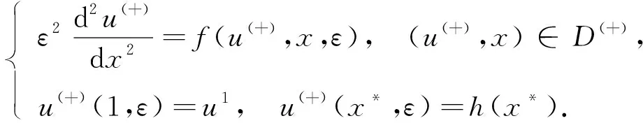
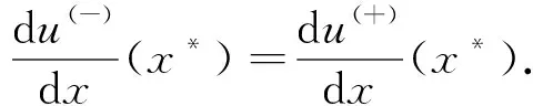
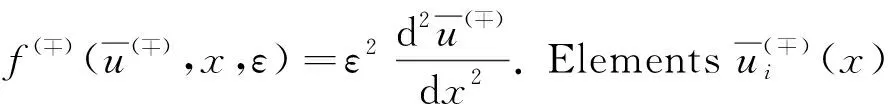
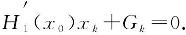
whereε>0 is a small parameter anduis an unknown function. We will build the solution of the problem (1) in the regionD={(u,x)|0 (2) wheref(∓)(u,x,ε) are sufficiently smooth functions and next inequality satisfies f(-)(h(x),x,ε)≠f(+)(h(x),x,ε). As you can see from the description of expression (2), we have two different areas in which the left and right solutions will be located. Often the boundary for these areas is a straight line. In this case, the area of definition of the left and right problems will be determined by a monotonically decreasing curveu=h(x),x∈[0,1]. The desired splitting for the regionDcan be written as Later in the article for elements describing the equations forD(-)we will use the symbol (-) and forD(+)we will use (+). In this work, we will study the existence of a solution of piecewise-smooth singularly perturbed problem (1) when there is exist an internal and boundary layers. For this reason, we need to introduce the following set of conditions. Fig.1 Solution of degenerate problem f(u,x,0)=0 Condition 1The degenerate equationsf(∓)(u,x,0)=0 have degenerate solutionsu=φ(∓)(x) which interact the functionu=h(x) at pointsx(∓), respectively. Given that the functionu=h(x) is monotonically decreasing, the inequalitiesx(+) Condition 2For the partial derivative of functionsf(u,x,0) the inequalities below should be satisfied Next, we consider the attached system for problem (1) as follows: (3) wherexis regarded as parameters. A basic phase analysis is required. It is clear that the associated equations have two equilibriums (φ(-)(x),0) and (φ(+)(x),0) forx∈[0,1]. According to Condition 2 they are both saddle points. Hence, forx∈[0,1], there exist stable and unstable manifolds for equilibrium (φ(-)(x),0). They have following expressions: In similar way, we can describe the stable and unstable manifolds for equilibrium (φ(+)(x),0) as follows: Based on all of the above-mentioned concepts, we can formulate the following condition. For convenience, we introduce the following notation: which satisfies following condition: Condition 4For allx∈[0,1], we requireH0(x)=0 holds. We can now proceed to construct an asymptotic approximation. In this part, we will deal with the construction of the asymptotical approximation for a contrast structure type solution of problem (1). To do this, we use the boundary function method and smooth matching condition. As usual, we assume the internal layer arises in the neighborhood of a pointx=x*wherex*∈[x(+),x(-)]. Based on the boundary function method, we can split the problem (1) into two new boundary value problems (4) and (5) Note that at the moment the value ofx*is not defined, so for convenience, we will look for it in the following form:x*=x0+εx1+…+εnxn+…. To find it, we can use the smooth matching condition: (6) The solutions of the boundary value problems (4) and (5) can be constructed in the form of the asymptotical approximationU(∓)(x,ε) as follows: (7) Here is regular parts, is internal layer parts,τ=(x-x*)/ε, is boundary layer parts,ξ-=x/ε,ξ+=(x-1)/ε. For expansions near the boundary value partsΠ(∓)u(ξ∓,ε) and the internal layer partsQ(∓)u(τ,ε), we need to introduce additional conditions: Next, we follow the basic algorithm of the boundary function methods. We use the asymptotical approximationU(x,t,ε) in the boundary value problems (4) and (5) and separate elements with different scale variables. Thus, we obtain a series of equations for finding the decomposition elements of the regular part, the boundary layer, and the internal layer. Now we need to solve all these equations. In the case of the internal layer partsQ(∓)u(τ,ε), we have the following problems: (8) (9) Note that at the moment we considerx*to be a fixed value. This is necessary to determine the general appearance of the solution in the internal layer parts. To simplify the writing of the equations, we introduce the following notation: Thus, the problems (9) can be rewritten in the form: (10) where Here and the functionsGk(x0)(k≥1) are known functions which containxi(0≤i≤k-1). According to Condition 4, we have a special case whenH0(x0)=0. Therefore, to findx0, we need the functionH1(x). In this case, the following condition holds: We just need to define the members of the boundary layerΠ(∓)u(ξ∓,ε). To do this, we have the following problems: (12) and (13) As you can see, they are quite similar to the equations that we used when constructing internal layers partsQ(∓)u(τ,ε). So we can use the similar methods to defineΠ(∓)u(ξ∓,ε). Thus, with sufficient smoothness of the functionsf(∓)(u,x,ε) andh(x), we can construct an asymptotical approximationU(∓)(x,ε) with internal layer in the transition pointx*up to the term ordern+1. It is worth noting that this approximation gives the accuracy of orderεn+1when substituting in equation (1). Let us denote Hence, we can obtain Theorem 1If Conditions 1~5 are satisfied, then the singularly perturbed problem (1) has a smooth solutionu(x,ε) with the following asymptotical approximation: In this article, the balanced case of a boundary value problem for nonlinear singularly perturbed differential ordinary equation is considered. We have considered a special case of this type of problem whenH0(x0)=0. The asymptotical approximation of solution is constructed and a new condition for determining the transition pointx*is derived. The existence of a smooth contrast structure type solution for the problem (1) has been proved. Our results can be applied in developing highly efficient numerical methods for solving similar problem.


2 Construction of a asymptotical approximation


2.1 The regular parts

2.2 The internal layer parts


2.3 The location of internal layer


2.4 The boundary layer parts

3 Existence theorem


4 Conclusions
猜你喜欢
华东师范大学学报(自然科学版)(2022年6期)2022-11-25数学物理学报(2022年4期)2022-08-22数学物理学报(2021年4期)2021-08-30中学生数理化·高一版(2021年2期)2021-03-19校园英语·下旬(2019年4期)2019-05-15校园英语·下旬(2019年4期)2019-05-15小学生学习指导(低年级)(2018年11期)2018-12-03中央民族大学学报(自然科学版)(2018年3期)2018-11-09校园英语·上旬(2018年7期)2018-09-08太空探索(2016年9期)2016-07-12
