
A Spatiotemporal Interactive Processing Bias Correction Method for Operational Ocean Wave Forecasts
2022-02-24 08:05AIBoYUMengchaoGUOJingtianZHANGWeiJIANGTaoLIUAichaoWENLianjieandLIWenbo
AI Bo, YU Mengchao, GUO Jingtian, ZHANG Wei, JIANG Tao, LIU Aichao,WEN Lianjie, and LI Wenbo
A Spatiotemporal Interactive Processing Bias Correction Method for Operational Ocean Wave Forecasts
AI Bo1), YU Mengchao1), GUO Jingtian2), *, ZHANG Wei2), JIANG Tao3), LIU Aichao2),WEN Lianjie2), and LI Wenbo2)
1) College of Geodesy and Geomatics, Shandong University of Science and Technology, Qingdao 266590, China 2) North China Sea Marine Forecasting Center of State Oceanic Administration, Qingdao 266100, China 3) 91033 Troops, People’s Liberation Army of China, Qingdao 266000, China
Numerical models and correct predictions are important for marine forecasting, but the forecasting results are often unable to satisfy the requirements of operational wave forecasting. Because bias between the predictions of numerical models and the actual sea state has been observed, predictions can only be released after correction by forecasters. This paper proposes a spatiotemporal interactive processing bias correction method to correct numerical prediction fields applied to the production and release of operational ocean wave forecasting products. The proposed method combines the advantages of numerical models and Forecast Discussion; specifically, it integrates subjective and objective information to achieve interactive spatiotemporal corrections for numerical prediction. The method corrects the single-time numerical prediction field in space by spatial interpolation and sub-zone numerical analyses using numerical model grid data in combination with real-time observations and the artificial judgment of forecasters to achieve numerical prediction accuracy. The difference between the original numerical prediction field and the spatial correction field is interpolated to an adjacent time series by successive correction analysis, thereby achieving highly efficient correction for multi-time forecasting fields. In this paper, the significant wave height forecasts from the European Centre for Medium-Range Weather Forecasts are used as background field for forecasting correction and analysis. Results indicate that the proposed method has good application potential for the bias correction of numerical predictions under different sea states. The method takes into account spatial correlations for the numerical prediction field and the time series development of the numerical model to correct numerical predictions efficiently.
numerical models; ocean wave forecasts; spatial interpolation; time series interpolation; successive correction
1 Introduction
Accurate information from marine numerical prediction is important to prevent and mitigate marine disasters and develop offshore engineering infrastructure. Marine numerical predictions to forecast future wind, SST, waves, and other variables are achieved through numerical modeling and observation of the actual conditions of the atmosphere and sea (Schulze, 2007; Pan, 2019). However, the results of numerical prediction are often quite different from the true sea state. Uncertainties always exist during numerical prediction because of errors associated with the numerical model and initial values used and the chaotic nature of atmospheric flow (Mass, 2002; Hart, 2004; Krishnamurti, 2004; Zhang and Pu, 2010; Wu, 2013; Chu, 2016). The bias of numerical prediction could directly affect the accuracy of marine fore- casts. Therefore, improving refined marine forecasting ability by correcting the bias of numerical predictions efficiently and enhancing the interpretability and applications of numerical models is of great importance.
Scholars at home and abroad have conducted numerous studies to improve the accuracy of numerical prediction and achieved remarkable results. Epstein and Leith first pro-posed the concept of ensemble forecasting, which changed the nature of forecasting from single-value certainty theory to multi-value probability theory, by assessing the influence of initial atmospheric values and uncertainties of numerical models on the forecasting results; the authors’ findings demonstrated good conformity with the reality of meteorological science and provided a new perspective for the development of other forecasting operations (Epstein, 1969; Leith, 1974). The development of statistical post-processing, data assimilation, and ocean observations has also provided accurate and reliable forecasts for marine decision-making (Cui, 2011; Bourgin, 2014; Guan, 2015; Chen, 2019; Bannister, 2020). Wang(2018) proposed a prediction-correcting frame- work by using a residual single hidden-layer feed forward neural network that could effectively correct the predicted consequences of significant wave heights in numerical models. Durai and Bhradwaj (2014) proposed four statistical bias correction methods, including running-mean bias correction, best easy systematic estimator, simple linear regression, and the nearest neighborhood weighted mean, for numerical prediction forecasts ofmaximumandmini- mumtemperatures.Duan(2017) proposed a new method of automatic model correction that could minimize the difference between predictions and observations by adjusting the parameters of the numerical weather prediction model. What greatly improves the accuracy of prediction is that the objective bias correction of numerical prediction results and the development of empirical methods can reduce the influence of model errors on prediction. Recent developments in the related technologies have enabled the construction of numerical models that are quite refined, with longer forecasting times and more objective forecasting results. However, errors in the accuracy of the numerical model due to the uncertainty of the model and the observed data are constantly noted (Hu, 2014). For example, using the results of numerical prediction to predict significant wave heights may not be effective because the physical mechanism of ocean waves is fairly complex (Wang, 2018; Liu, 2019; Yang, 2019a; Chattopadhyay, 2020). Thus, forecasters are still indispensable in current wave forecasting activities.
The ocean is a highly complex and nonlinear dynamic system. Some limits to the predictability of the ocean exist (Wang, 2014). Manual prediction cannot be completely replaced by numerical prediction because forecasters must conduct a final check on numerical prediction products. Manual prediction corrects the results of marine prediction according to numerical predictions using manual experience and real-time observations to determine the trends of sea states. Manual correction relies on forecasters’ historical experience of the accuracy of numerical forecasts and scientific analysis of changes in weather processes, especially for specific sea areas and ocean elements. Marine forecasting is developing toward intelligent gridded forecasting with refined contents and seamless space-time relations (World Meteorological Organization, 2015; Jin, 2019). Combining the experience of forecasters with numerical predictions is a current trend. High-quality numerical prediction products can be used to revise intelligent gridded forecasting methods and interpret interactive prediction platforms, which can be combined with ocean observations and the experience of forecasters to improve prediction accuracy (Du, 2013).
The use of the appropriate correction method is key to ensure the efficiency and accuracy of prediction correction, and an intelligent interactive platform is a prerequisite for forecasters to make manual corrections. The Advanced Weather Interactive Processing System developed by the National Weather Service uses the Graphical Forecast Editor to implement gridded forecasting editinghuman-computer interaction, thereby allowing forecasters to modify the forecast value of each element directly using rich graphical tools (American Meteorological Society, 2002; Mass, 2003). The correction method provided by the system is intuitive and easy to understand. However, during actual implementation, the workload of fore- casters is extremely heavy; thus, the method is generally used for the detailed correction of sensitive weather elements. The Meteorological Information Comprehensive Analysis and Processing System is an intelligent gridded forecasting platform developed by the National Meteorological Centre of China. It realizes single-point and regional editing and modification of the original grid field and retrieves the deformation results of the isoline back to the grid field to correct the forecasting field (Gao, 2014; He, 2018). The system meets the correction requirements of a single field and a single time for the forecasting fieldthe diversity method, but it does not consider the correlations of spatiotemporal data. Thus, this system is unable to analyze the continuity of forecasting elements in the time dimension. Further development of the operational level of marine predictions with the continuous upgrade of marine forecasts is necessary, and the selected forecasting platform must provide refined gridded forecast production. At present, research on intelligent gridded forecast correction is scarce. The traditional forecast correction method mainly focuses on the forecast correction of observation stations and seldom takes into account the correlation between the time series of forecast fields; thus, satisfying the requirements of current wave forecasting is challenging (Yang, 2019b).
Forecasters can effectively overcome the scientific prob- lems of objective forecasting by finding defects and then constantly improving the forecasting level, thus supporting the further development of subjective and objective fusion forecasting products. Aiming to address the demands of operational wave forecasting correction and pro- duct release, this paper carries out research on grid forecast correction algorithms and technologies by making full use of the advantages of forecasters in marine forecasting. This paper develops a forecast correction technology based on the subjective and objective fusion of the grid data of numerical prediction and the forecasting experience of forecasters to realize the simple and efficient correction of objective forecasting bias. By analyzing the spatiotemporal correlations of the numerical wave model, this paper proposes a spatiotemporal interactive processing forecast bias correction method based on subjective and objective fusion to improve the efficiency of forecasting correction. This method combines the advantages of numerical prediction and Forecast Discussion. In Forecast Discussion, forecasters construct forecasting conclusions after discussing the development of future weather and its basis when making weather forecasts. This approach provides an efficient means to input manual experience into the computer to realize automatic correction. First, the spatial trend is adjusted by spatial interpolation of the spline with barriers based on results of the Forecast Discussion. Then, statistical analysis and spatial processing are conducted by analyzing the spatial correlation of grid data in the interpolation field and its adjacent regions to achieve coordination and consistency in the forecast field. Finally, the correction results of the spatial field are interpolated to the adjacent numerical prediction field by successive correction analysis. The proposed method is subsequently applied to the actual bias correction of significant wave height predictions for marine waves from the European Centre for Medium-Range Weather Forecasts (ECMWF). This method is mainly applied to the production and release of daily operational wave forecastingproducts after Forecast Discussion. The forecasting results obtained in this manner may be expected to be more reasonable and accurate. The proposed method can compensate for the disadvantages of numerical models in operational forecasting by combining the experience of fore- casters to correct numerical predictions and develop subjective and objective fusion forecast correction technology. Forecasters especially have advantages on correctly judging the process of marine waves and correcting the re- sults of numerical prediction under extreme-causing weath- er patterns.
2 Materials and Processing Method
2.1 Research Area and Materials
The prediction data used in this paper are the significant wave height predictions of numerical models obtained from the ECMWF. The range of the wave field in the Yellow and Bohai Seas selected for model analysis is 33.69˚N–40.94˚N, 117.41˚E–127.36˚E, as shown in Fig.1. The spatial resolution of the numerical model is 0.25˚×0.25˚, and the useful forecasting time can reach 240h. The time resolution of the forecast data ranging from 0h to 72h is 3h, while that of data ranging from 72h to 240h is 6h. The daily start time of the forecast is 20:00 (Beijing time, the same below). Fig.1 shows the distribution of buoy stations in the Yellow and Bohai Sea areas. A total of 10 buoy stations are selected as observation points to verify the applicability of wave forecasting data correction, and the number of buoys in each region is shown in Table 1. This paper selects 24-h forecasting data (the time range is shown in Table 2) and the buoy station observation data for analysis and correction. The weather conditions on November 17–18, 2019, include cold air and cyclone.
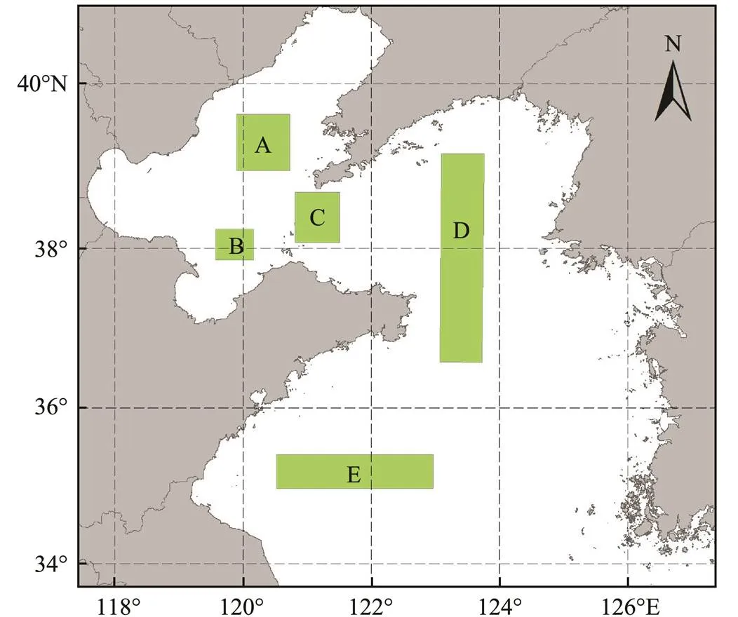
Fig.1 Study area and buoy distribution.
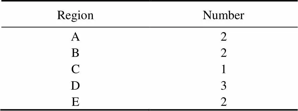
Table 1 Number of buoys in each region
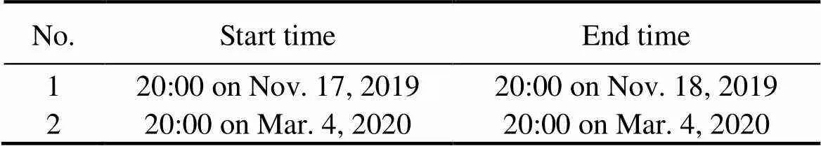
Table 2 Data time range
2.2 Data Preprocessing
The data from numerical models must be converted into vector and raster data that are easier to process, thus providing basic data for human-computer interaction prediction. The spatiotemporal interpolation algorithm is simultaneously used to improve the resolution of the forecasting data to satisfy the requirements of the experiment.
The resolution of numerical models may be improved by spatiotemporal downscaling for refined gridded forecasting (Ben Alaya, 2015; Tang and Bassill, 2018). The numerical prediction field (NPF) is resampled by bilinear interpolation to improve spatial resolution (Goyal, 2018). Time series interpolation is used to interpolate the intermediate time data (interval, 1h) to improve the temporal resolution. When an obvious bias is observed between the numerical forecasting results and the sea state, the forecaster corrects the former at a specified time by adjusting the isoline trend and combining spatiotemporal interpolation. The required data are divided into two types: the raster data of NPF and the vector data of the isoline.
The numerical prediction data must be preprocessed before application. First, the numerical prediction gridded values in the study area are loaded, the raster dataset is created, and the unit values are written to obtain the original-resolution NPF data. NPF data with a resolution of 0.025˚×0.025˚ are obtained by bilinear interpolation to produce the original-resolution NPF raster data. Then, NPF data with a temporal resolution of 1h are obtained by time series interpolation. Finally, the vector data of the isoline are extracted and processed on the basis of the numerical predicted field raster data after specifying the starting isoline and isoline spacing. The isoline processing methods include, among others, curve simplification, smoothing, topological intersection processing, and elimination of lines that do not meet the requirements.
The bilinear interpolation algorithm uses the weighted average of the values of the four nearest grid points on the original grid to obtain a new value of the output unit (Li and Liu, 2018; Rukundo and Schmidt, 2018). The resulting grid surface is smoother and has good continuity. The bilinear interpolation of regular grid data improves the spatial resolution and quality of the extracted isoline data. The curve is smoother and no obvious sharp occurs at breakpoints.
The forecasting time of the ECMWF numerical model data used in this paper from 0 to 72h, whose time interval is 3h. The prediction field data at adjacent moments are used to interpolate the missing forecasting time and improve the temporal resolution of the data. The equation of time series interpolation is as follows.
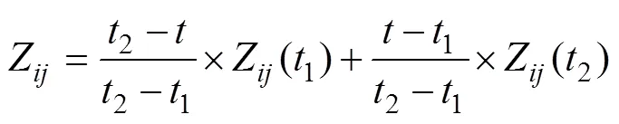
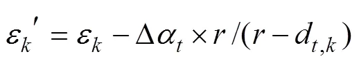
where Z() represents the estimated grid points of the interpolation field in rowand columnat time,1and2are the time values of prediction fields adjacent to the interpolation time, and Z(1) and Z(2) represent the grid point prediction values of the corresponding grid field in rowand columnat time1and2, respectively.
The experimental data are preprocessed as follows; here, the practical application demands of daily forecasts of significant wave heights are taken as an example. Bilinear and time series interpolations are applied to the NPF in space and time to obtain forecast data with a spatial resolution of 0.025˚×0.025˚ and a time resolution of 1h. The method improves the spatiotemporal resolution of the grid data and meets the requirements of operational forecasting. Fig.2 shows a rendering of the NPF before and after bilinear interpolation at 20:00 on March 4. The grid spacing is reduced by bilinear interpolation, and the visual impression of the raster map is smoother after interpolation. As shown in Fig.3, the bilinear interpolation of the wave field can improve the spatial resolution and has little effect on the accuracy of the forecasting data. The isoline data of significant wave heights are then extracted at 0.5m intervals using the NPF with a spatial resolution of 0.025˚×0.025˚; here, the value of the initial isoline is 0m. The isoline data are superimposed as a layer and displayed above the raster layer in the operational applications of prediction correction. Furthermore, the numerical prediction results are analyzedmanual correction based on the trend of isoline data.

Fig.2 Results of bilinear interpolation.
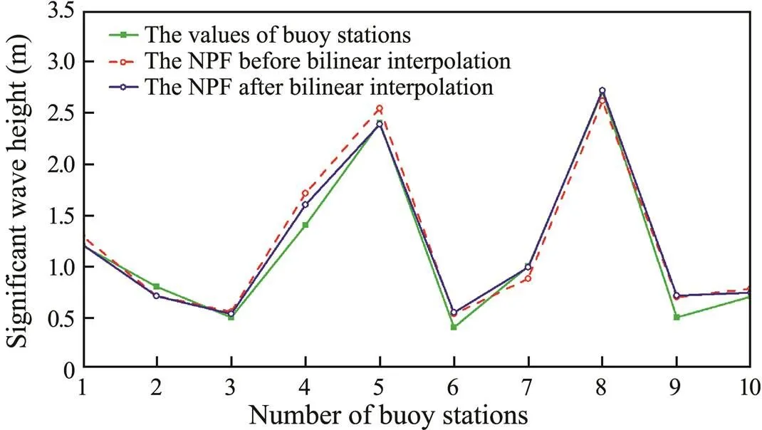
Fig.3 Accuracy analysis of bilinear interpolation.
3 Spatiotemporal Interactive Correction
3.1 Overview
The interactive process of the proposed correction me- thod is mainly reflected in the forecaster’s judgment of the overall trend of the wave forecasting process and the setting of the influence weight of the time series. The single-time numerical prediction field is corrected on the basis of the spatial correlation of marine wave forecastsby editing the trend of isolines, including human-computer interaction, spatial interpolation, and sub-zone statistical analysis. Numerical predictions are generally accurate in time trends. Therefore, this paper proposes a time series prediction correction method to correct temporal forecasts with the aim of maintaining the temporal developmenttrend of the original numerical models to improve the efficiency of forecast correction. The time series prediction correction method sets the influence radius considering the wave forecast process to expand the spatial correction results to the adjacent time prediction by successive correction analysis. Finally, multi-time spatiotemporal forecasting data correction is completed, as shown in Fig.4.
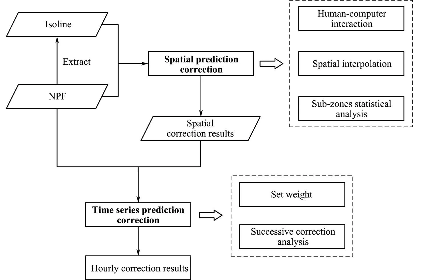
Fig.4 Spatiotemporal interactive correction.
3.2 Spatial Prediction Correction
3.2.1 Overview of the correction process
The spatial prediction correction method proposed in this paper involves spatial interpolation and sub-zone numerical analysis. In the actual operational task, the raster data of the NPF are rendered according to the specified interval, and the corresponding time vector data of isoline is displayed as a layer overlay above the raster data. The NPF matches the isoline data, as shown in Fig.5. First, the iso- line trend was adjusted by editing nodes or adding, deleting, and moving isoline when an obvious bias between the numerical and manual prediction results is found. Then, the control points of the isoline are used as input points for spatial interpolation to obtain the spatial interpolation field considering manual intervention (SIFCMI). Fig.6 shows the spatial distribution of control points extracted from the isoline shown in Fig.5. The smooth grid surface, which is obtained by using splines with barriers for spatial interpolation, can simulate the spatial numerical distribution of marine elements to a certain extent. However, given the sparse isoline distribution, the effect of regional interpolation is relatively poor. Thus, sub-zone numerical analysis is necessary to correct outliers in the interpolation field due to the influence of the interpolation algorithm and the spatial distribution of control points.
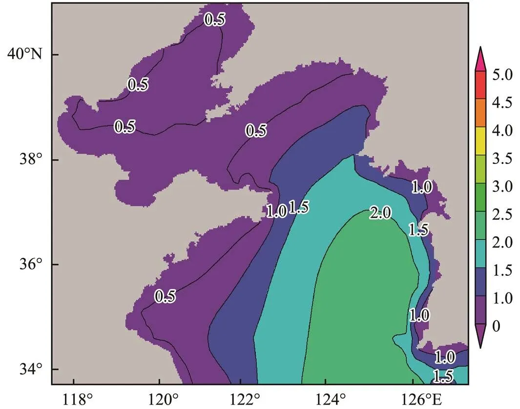
Fig.5 Vector and raster data.
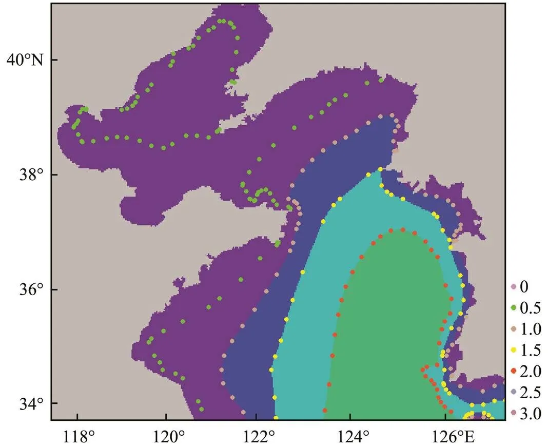
Fig.6 Spatial distribution of control points.
Sub-zone numerical analysis correction is performed to correct regional outliers and enhance the coordination and consistency of spatial data. First, the SIFCMI is partitioned through the isoline. The partitioned area is then divided into large and small correction areas for separate processing according to the spatial relationship between the SIF- CMI and the isoline. The large correction area refers to a field area bounded by the editing isoline; the boundary isoline that makes up the small correction area is not adjusted by manual trending. The small correction area is adjusted in terms of the overall trend by the difference between the NPF and spatial interpolation field (SIF), and the large correction area is analyzed on the basis of the outliers. The SIF refers to the interpolation field obtained by directly extracting and interpolating the control points of the original isoline using spline interpolation with barriers. After processing these two areas, regional numerical statistical analysis is performed to ensure that the values of each region are distributed within the same range. Spatial interpolation is combined with sub-zone numerical analysis correction to obtain the spatial prediction correction field (SPCF) and realizes the correction of single-time numerical model prediction results. The detailed process is shown in Fig.7.
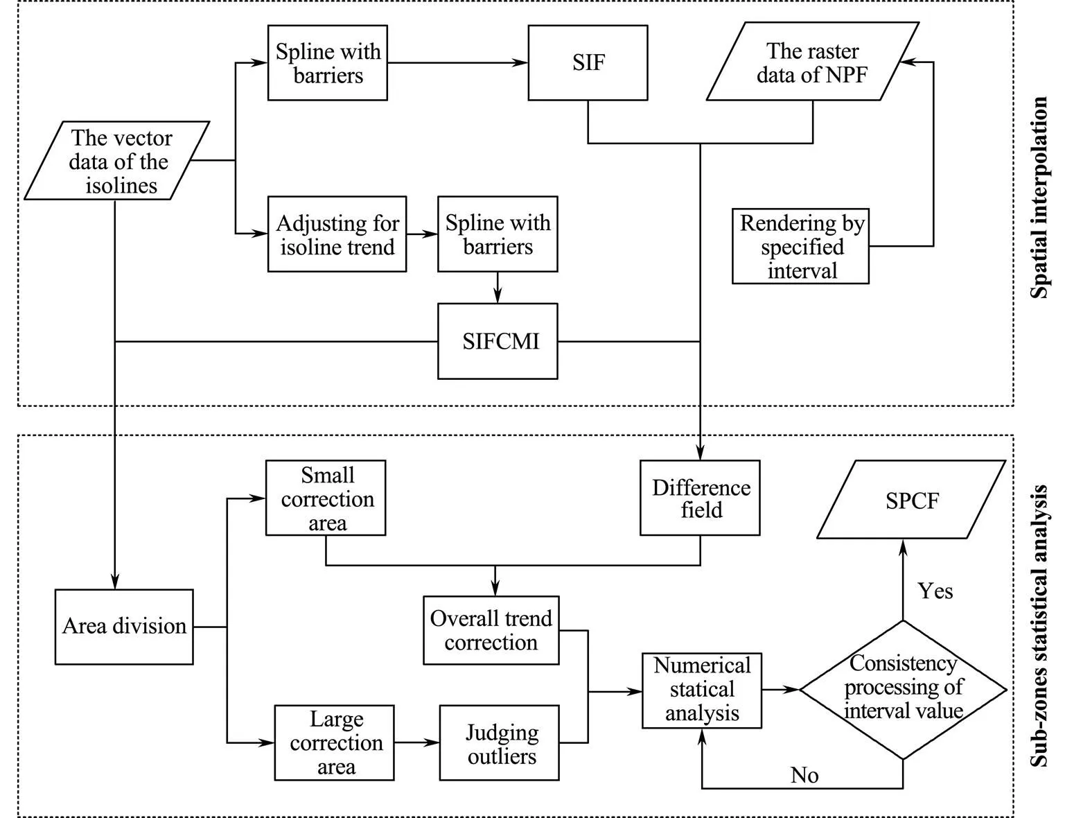
Fig.7 Spatial prediction correction.
3.2.2 Spatial interpolation correction
Spatial interpolation is a method of transforming discrete and irregular observation data into regular grid data. Common spatial interpolation methods for meteorological elements include the Kriging method, the inverse distance weighted (IDW) method, spline interpolation, polynomial interpolation, Cressman objective analysis, and the Delaunay triangulated method (Irmak, 2010; Liu, 2011; Yu, 2017; Fei, 2018). Spatial interpolation methods for different spatial variables generally differ, and the effect of the same interpolation method is relative even for the same spatial elements because of the influence of geographical distribution and space-time scale (Zhang, 2015; Susanto, 2016). In other words, the optimal interpolation method does not exist. Therefore, using the appropriate spatial interpolation method is key to ensure the effect of spatial interpolation.
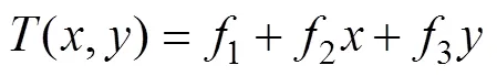
In this paper, the control points from the isoline were input into the interpolation function in which the boundary line features of the study area were considered barriers to construct the SIFCMI through spline interpolation with barriers and simulate the spatial numerical distribution of the marine prediction field. The spline method mini-mizes the total surface curvature used to estimate the camber value, which fits a continuous smooth surface through discrete point data. The expression for the interpolation of the spline function is as follows (Li, 2010):
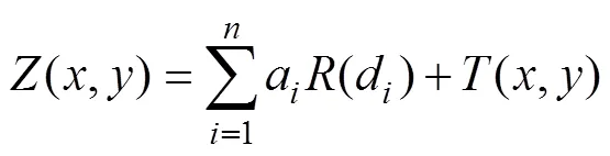
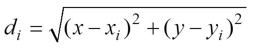
where() is the estimated value of the interpolation feature,is the number of discrete points involved in interpolation,arefers to coefficients found by the solution of the linear system of equations, anddis the distance from point (,) to the known point.(d) and(,) are described in Eqs. (4) and (5):
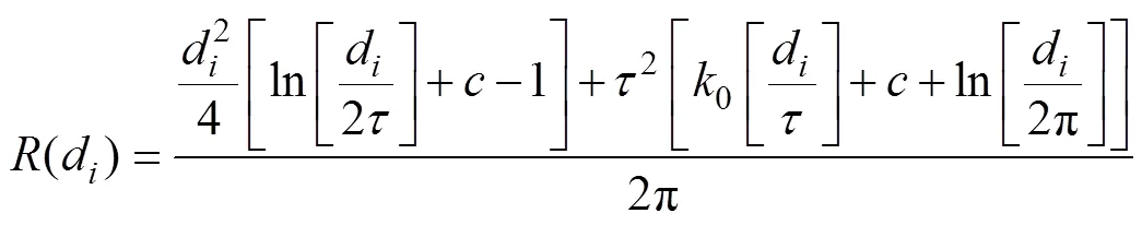
In Eq. (4),2is the weight coefficient, which defines the weight of the third derivatives of the surface in the curvature minimization expression. The higher the weight, the smoother the output surface. The values entered for this parameter must be equal to or greater than zero. The typical values that may be used are 0, 0.001, 0.01, 0.1, and 0.5.0is the modified Bessel function, andis a constant. In Eq. (5),fare coefficients found by the solution of the linear system of equations.
The correlation coefficients1,2,3, andaare determined by the following linear system of equations:
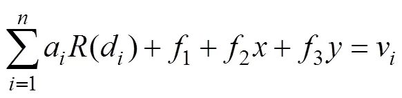
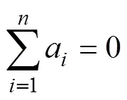
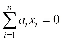

wherevis the value of the control point. The calculation of coefficients requires the simultaneous solution of Eqs. (6)–(9).
This paper compares spline interpolation with barriers with kriging interpolation and IDW according to the discrete points shown in Fig.6. As shown in Fig.8, the interpolation results of the kriging and IDW methods are quite different from the original forecast field in the closed area of the isoline. The two methods cannot simulate the numerical distribution trend of the original gridded field. In operational applications, the interpolation results must retain the distribution characteristics of each zone to satisfy the requirements of sub-zone forecasting correction. Therefore, this paper used spline interpolation with barriers to simulate the numerical prediction field in the spatial correction process.
Spline interpolation with barriers applies a minimum curvature method that takes into account the input point data encoded in barriers and surface discontinuities during surface fitting by the spline function (Terzopoulos, 1988; Smith and Wessel, 1990; Zoraster, 2003; Briggs, 2012). Some sample points that are closer in space show astrong correlation when interpolating an irregular research area. However, these points may not actually be related to each other when the influence of many factors in the actual situation is considered. For example, the same marine elements affected by topographic factors may be independent or different on the left and right sides of the land when the adjacent sea area is spatially divided by land. When combined with the analysis of the actual terrain, the addition of barriers can effectively solve the problem where the sample points are adjacent in space but have no spatial correlation during the interpolation process, therebyimproving the interpolation effect. In particular, this paper sets the boundary of the study area as obstacle elements to avoid the influence of terrain factors on spatial interpolation. Through the above analysis, spline interpolation with barriers can better simulate the sea state distribution characteristics of the study area.
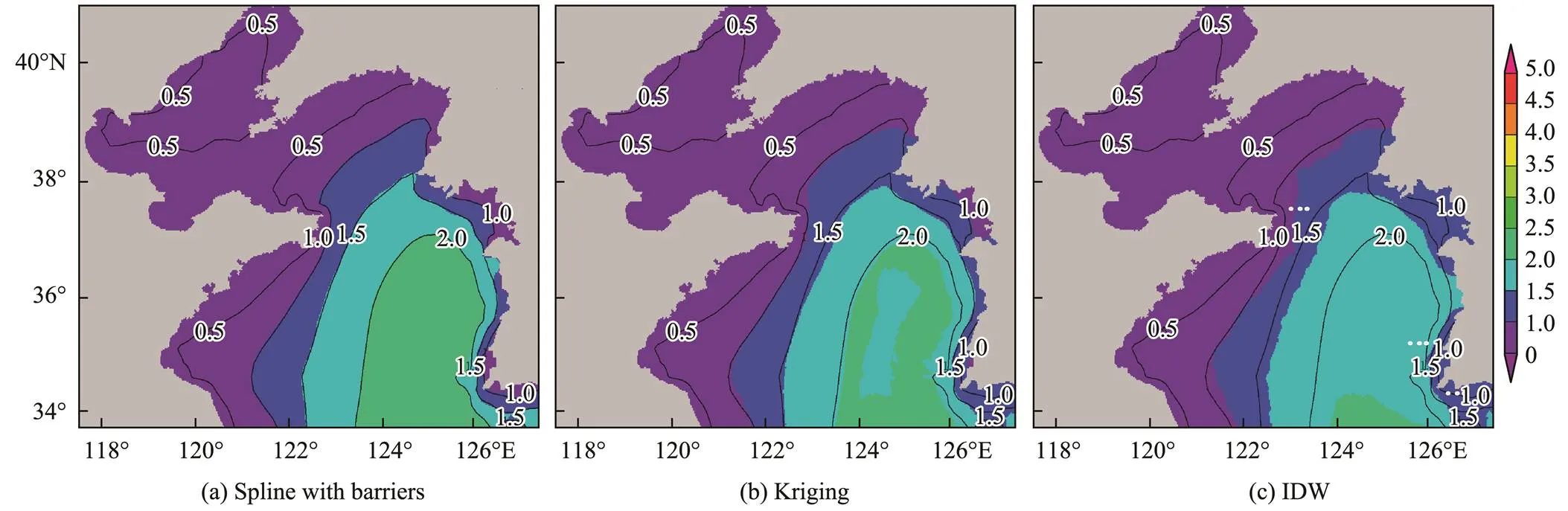
Fig.8 Comparison of different interpolation methods.
3.2.3Sub-zone numerical analysis
The spatial interpolation correction method produces a new spatial field according to the spatial distribution of the isoline; this field is able to reflect the spatial distribution of marine elements to a certain extent. However, the interpolation method cannot completely explain the actual ocean conditions and the physical laws of ocean elements, thus featuring a certain degree of uncertainty. In addition, the accuracy of spatial interpolation is influenced by factors, such as the appropriate number of interpolation points and the uniform distribution of control points. This paper proposes a method to improve the interpolation accuracy and render the numerical distribution of the SIFCMI more in line with the sea state of marine elements. Specifically, the difference field between the SIF and NPF is used to conduct numerical statistical analysis of the SIFCMI.
First, the SIFCMI was divided into areas with boundaries composed of the isoline or the boundary lines of the study area. The region adjacent to the artificially adjusted isoline is then defined as the large correction area, the spatial field of which is greatly affected by spatial interpolation correction values when the isoline trend is adjusted according to the topological relationship between the isoline and each regional surface. The other areas are small correction areas with space fields that are relatively less affected by the spatial interpolation correction values. The isoline comprising the large correction area boundary is inconsistent with the original isoline in terms of spatial distribution after the trend is adjusted manually, thereby resulting in a low correlation between the interpolation results and NPF. Because the isoline of the small correction area is not adjusted manually, the distribution of the extracted control points is consistent with the corresponding gridded data of the NPF, and an obvious correlation between the SIF and NPF in the numerical distribution may be observed.
The numerical forecast field has obvious correlation before and after correction; thus, trend adjustment and outlier treatment were used to adjust the regional values of the SIFCMI. The spatial field in the small correction area is only slightly affected by isoline trend adjustment in which the boundary isoline was not manually adjusted, thereby indicating that the spatial numerical distribution in this area is consistent with the actual distribution of marine elements after analysis by forecasters. However, the bias between the SIF and NPF is observed in the small correction area because an accurate understanding of the actual forecast correction needs cannot be achieved by any spatial interpolation method. The bias mainly refers to the influence when the spatial field changes in the surrounding area. If the bias is beyond a specified tolerance, the spatial interpolation method is considered unreasonable for the estimation of spatial values in this area. According to the above analysis, the overall trend correction of the SIFCMI is conducted using the correlation between the SIF and NPF. The spatial field takes into account the numerical influence caused by the variation of the surrounding regional field and the rationality of the numerical prediction results. The correction equation of the small correction area is as follows.
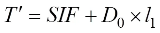
whereis the result of the spatial correction,0represents the difference field between the NPF and SIF, and1is the correction coefficient. The expressions of0and1are as follows.
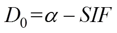
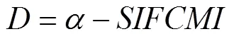
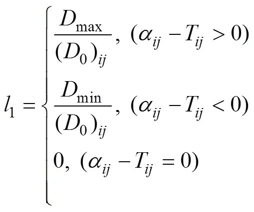
whererepresents the difference field between the NPF and SIFCMI,maxandminrespectively represent the maximum and minimum values of the difference fieldin the correction area, (0)represents the value of0in rowand columnof the corresponding spatial position when the difference fieldtakes the maximum or minimum value, andandTare the gridded values on the specified row and column number.
The spatial field of the large correction area corresponds better to the sea state distribution after manual adjustment. However, outliers due to the influence of the spatial interpolation algorithm and spatial distribution of sample points are also observed. The method of judging outliers is as follows. First, the numerical range of the SIFCMI is divided by the value and distribution of the isoline. Then, all gridded values in the large correction area are read to determine in which interval the gridded values are mainly distributednumerical statistics in the area. The spatial characteristics of the region are mainly concentrated in this closed interval [a, b], while the values outside the interval [a, b] are considered outliers. The outliers are determined, and the whole SIFCMI is continuously analyzed and corrected region by region so that the values of each region are consistently in the interval range. The outliers are assigned to be the maximum or minimum value of the non-abnormal value for the gridded data that still do not meet above conditions. Consistency processing of interval values conform to the correlation between spatial data and improves the rendering graphics effect of the spatial prediction field.
3.3 Time Series Prediction Correction
3.3.1Overview of the correction process
The spatiotemporal data of significant wave heights show strong correlations in space and have obvious time series characteristics. When the results of numerical prediction at a certain time are corrected, the spatial fields of the adjacent time should be adjusted according to the correlation of the time series data and the time development trend of numerical model data. However, forecasters are unable to correct the forecast field hourly because of the requirement of forecast timeliness in the production and release of operational ocean wave forecasting products. This paper proposes a multi-field linkage editing algorithm for time fields based on the results of spatial prediction correction to achieve efficient human-computer interaction in the production of forecasting products. The method analyzes the continuity of numerical prediction results in time by combining the spatiotemporal characteristics of the time series between SPCF and NPF. Then, the analysis increment is interpolated to the adjacent time series by successive correction analysis (Benjamin and Seaman, 1985). Finally, the linkage correction of multi-time prediction data is realized with minimal changes to the time development trend of the numerical model. In this paper, successive correction analysis is applied to the temporal interpolation process. The NPF data are taken as the initial value field, and the difference between the SPCF and the initial value field is used to correct other NPF at different times. Then, the difference between the new field and corresponding NPF is calculated. The final new field is corrected until the corrected field approximates the spatial correction value considering the time influence radius. The method considers the correlation of the spatiotemporal data and the development trend of the numerical wave model to realize the efficient correction of the results of the numerical prediction time series with small errors; the relevant principle is illustrated in Fig.9.
3.3.2 Time series prediction correction
The NPF was used as the background field for successive correction analysis. First, the time series dataset of the NPF [0,1,···,,···,−1] and the spatial dataset of the SPCF at the adjacent time [I,II,···,,···,], whererepresents the NPF of significant wave height at time, 0<£−1,is the correction field of spatial prediction at time, and 0<£<, were loaded. Then, the difference between the correction field of spatial prediction and theNPF was calculated. The time series dataset of the difference field [I,II,···,, ···,] was obtained, whererepresents the difference field between the SPCF and the NPF at time. The expression ofis as follows.
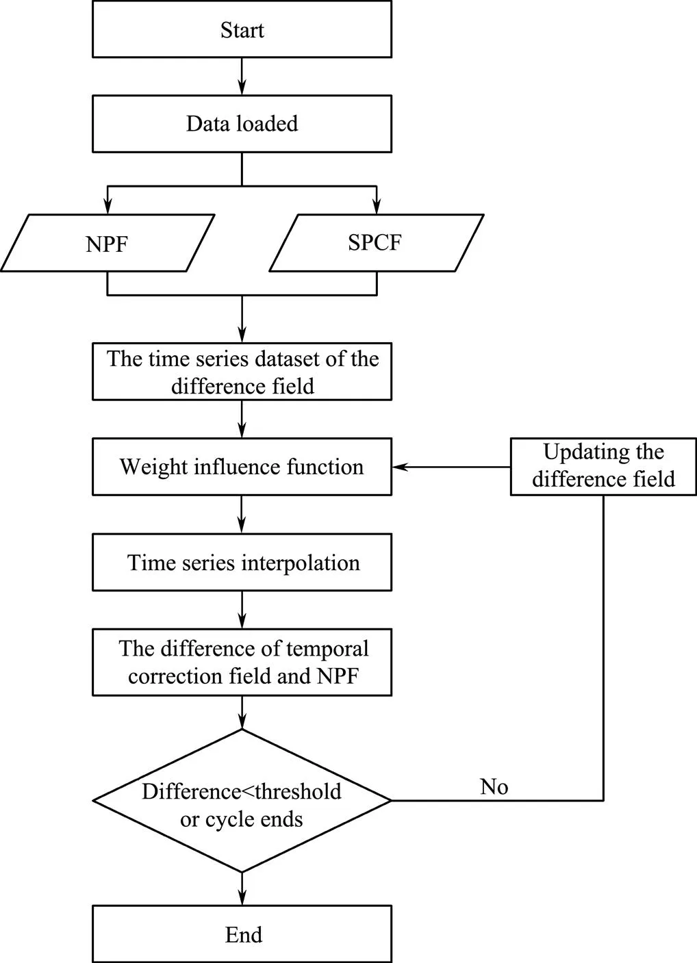
Fig.9 Time series prediction correction.

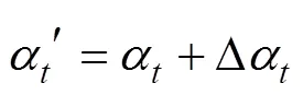
The weight influence functionW, kwas set for time series interpolation. The equation ofW, kis as follows:

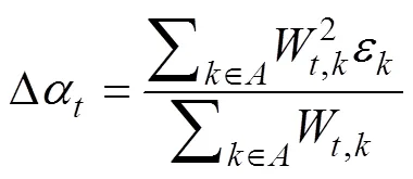
whererepresents the time of the NPF,represents the time of the SPCF,d,=|–|represents the time interval between the NPF to be corrected in time and the SPCF, andis the influence radius of interpolation. Specifically,can be calculated according to the actual ocean situation and adjusted according to the effect of time series interpolation. The weight influence function is brought into the time series interpolation to obtain the dataset of the time series correction field [0,1,···,,···,−1]. The equation for interpolation is as follows:
whereDrepresents the difference between the time series correction field and the NPF. The equation ofDis as follows.
whereis the time set of the SPCF. The convergence threshold is set; ifDis less than this threshold or the cycle reaches a specified number of times, the correction ends. If the end condition is not satisfied, the difference field is updated to obtain a new sequence, and the cyclic regression correction of the NPF continues. The expression for updating the difference field is as follows.
The spatial variation of the NPF is interpolated to the adjacent time series by prediction correction for the time series. The proposed method does not change the evolution law of the numerical mode overall, but the time series data are changed smoothly during interpolation. More- over, the algorithm is efficient and can realize the accurate correction of continuous multi-time prediction data.
4 Results and Discussion
4.1 Evaluation Indices
The prediction of significant wave heights of the ECM- WF is analyzed using the above correction method with the time ranges shown in Table 2, Nos. 1 and 2. In this paper, the data from the ocean buoy stations are taken as the observation data. Root mean square errors (RMSEs), maximum forecast errors (MFEs), and correlation coefficients (CORs) are used to measure the applicability of the method, the spatial correlation, and the stationarity of time series during the correction. The calculation equations for the above three statistics are as follows.
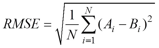
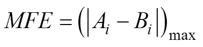

whereArepresents the prediction value of significant wave height,`is the mean of the prediction values,Bare the observation data from the buoy stations,`represents the average value of observations from the buoy stations, andis the total amount of data.
4.2 Spatiotemporal Prediction Correction
Interpolation correction of the spatiotemporal data of the numerical wave predictions is conducted using historical observations and other supporting materials in combination with the professional knowledge and experience of forecasters. Analysis of the numerical prediction results by forecasters reveals obvious bias between the numerical predictions and the actual marine conditions at 3:00, 14:00, and 20:00 on March 5. First, the isoline trend is adjusted to the judgment state. Then, the control points of the isoline are extracted for spline interpolation with barriers to obtain the SIFCMI. Thereafter, sub-zone numerical analysis of the SIFCMI is carried out region by region. Finally, spatial prediction correction of the numerical prediction at the corresponding time is completed. Fig.10 shows the numerical prediction fields before and after spatial prediction correction and the difference fields obtained at 3:00 (a), 14:00 (b), and 20:00 (c) on March 5, 2020; here, ais the result before correction, bis the result after correction, and c=b–a.
The time series data of the NPF are analyzed and corrected using the spatiotemporal correlation of wave data. First, the hourly data of NPF from 0h to 24h and the data of SPCF at three specific times are loaded. Next, the difference field of the time series is obtained by calculating the difference between the SPCF and the corresponding NPF. Then, it is analyzed that the spatial distribution state and prediction accuracy of the prediction field at the adjacent time in the calculation of weight influence function. The interpolation influence radius of 3:00 on March 5 is set to 1, and the influence radii of 14:00 and 20:00 are set to 8. The weight influence function is subsequently substituted into the time series interpolation function to perform four cyclic corrections. Finally, the difference field is updated by successive correction to realize the linkage correction of the time series data.
In a normal wave climate, forecasting correction is used to verify the stability of the algorithm and whether a large error is caused by manual intervention in the spatial value of the forecast field. The results of wave forecasting under special weather conditions are analyzed in this paper by taking wave forecasts under cold air and cyclone as an example (time range, Table 2, No. 1). Spatial correction of the NPF at 8:00 on November 18, 2019, is performed, as shown in Fig.11. The influence radius of the interpolation is set to 21 to achieve the linkage editing of the time series data during time series interpolation. The radius is determined by the forecaster according to the results of the Forecast Discussion.
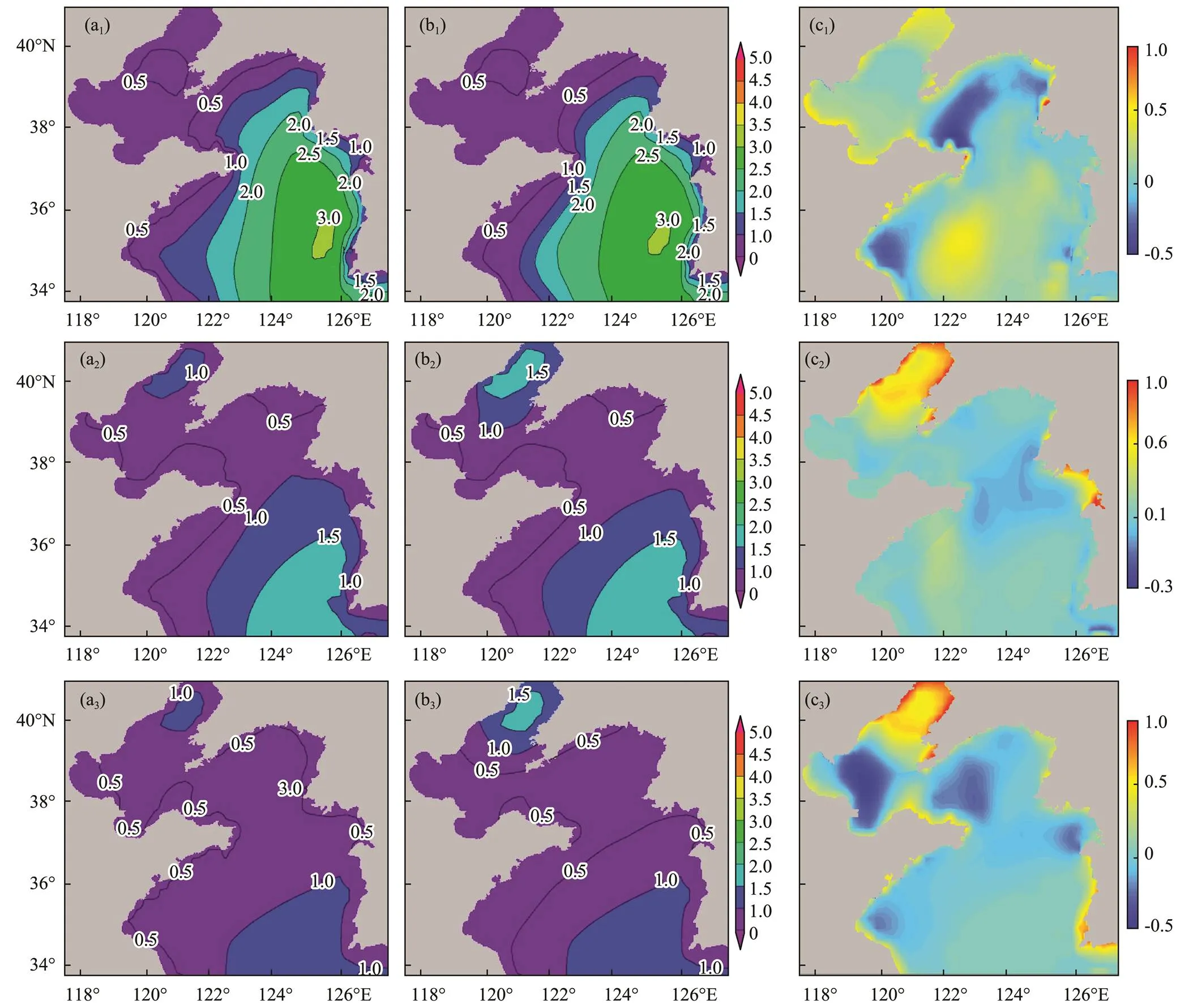
Fig.10 Accuracy analysis of spatial prediction correction in a normal wave climate.
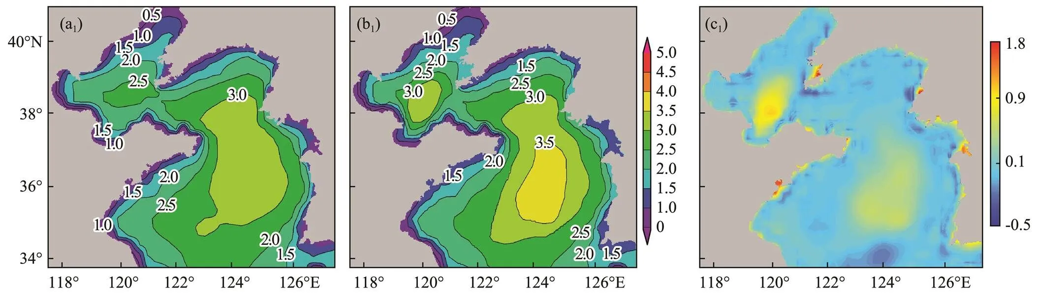
Fig.11 Accuracy analysis of spatial prediction correction under cold air and cyclone.
4.3 Discussion
The gridded point values of the NPF and corresponding correction field are extracted according to the position of the buoy stations. Then, the RMSE, MFE, and COR between the prediction values of significant wave height and the observations from the buoy stations before and after correction are calculated. According to statistical analysis in Table 3, the maximum prediction error and RMSE between the predicted value of the significant wave height and the observations from the buoy stations are reduced from 0.42–0.57m to 0.21–0.22m after spatial correction for the forecasting results at 3:00, 14:00, and 20:00 on March 5, 2020. The CORs at these three moments improved after correction compared with those obtained before correction, especially at 20:00 on March 5; in particular, COR increased from 0.53 before correction to 0.97 afterward. This result indicates that the bias correction results of significant wave height are more consistent with the actual marine conditions obtained from the buoys compared with the actual observations at 20:00 on March 5, 2020, as shown in Fig.12.
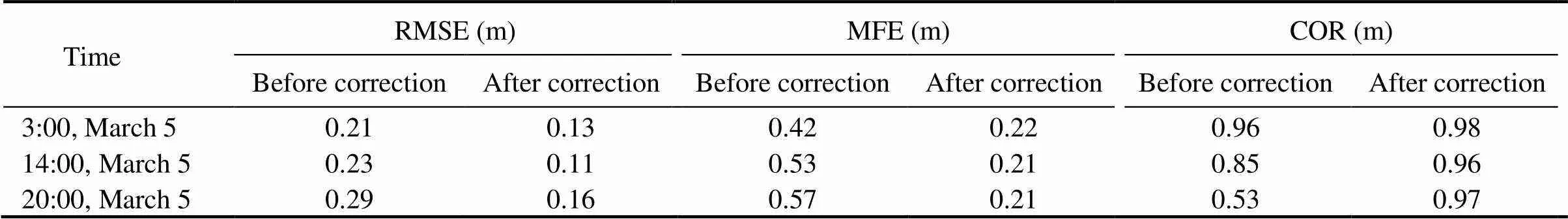
Table 3 RMSEs, MFEs, and CORs between the significant wave height predictions and buoy station observations

Fig.12 Accuracy analysis of SPCF.
Fig.13 and Fig.14 respectively show the time series of the RMSEs and MFEs between the significant wave height predictions and the buoy observations before and after correction (time range, Table 2, No. 2). In Fig.13 and Fig.14, the RMSEs between the significant wave height predictions and the buoy station observations are generally small, while the MFEs from the 16th hour to the 24th hours are between 0.35 and 0.6m. In this experiment, the numerical prediction results of the 7th, 18th, and 24th hours (, 3:00, 14:00, and 20:00 on March 5, 2020) are corrected in space based on the forecasters’ analysis. The linkage correction of the other moments from the 12th hour to the 24th hour is corrected by time series prediction correction. The curves in Fig.13 and Fig.14 show that the RMSEs and MFEs decreased significantly at multiple moments compared with those obtained before correction. The influence ranges of ocean observations and spatial correction results in time are analyzed during time series interpolation, and the influence radius of time interpolation is set. Because the forecasting result at the 7th hour is quite different from the manual prediction, the time interpolation influence radius at this moment is set to 1. The forecasting results at the 18th and 24th hours and their neighboring moments are all quite different from the corresponding manual predictions, so the influence radius is set to 8 after considering the spatiotemporal correlation of the wave data and the interpolation effect. Thus, the automatic correction of the adjacent time series data is realized using the manual correction field.
In this paper, the spatial distribution characteristics of the NPF are completely considered during spatial prediction correction. Spatial interpolation takes isoline control points as input points; the isoline is extracted from the numerical prediction field, so these control points retain the spatial distribution characteristics of the original numerical prediction field. The spline interpolation algorithm also considers the spatial distribution of discrete points. Finally, the interpolation results show good stabil- ity, generate only a few outliers, and reflect good spatial correlations with the original prediction field. General interpolation methods are easily affected by human intervention in uncorrected sub-regions when the overall wave height is low or the isoline distribution is sparse, resulting in errors or outliers. Verification of wave height forecasts in the absence of special weather confirms the stability of the proposed method for bias correction under normal weather conditions. The interpolation process is divided into two steps: overall estimation and sub-region analysis. Overall trend correction in other areas will not cause outliers after bias correction is completed. The ECMWF data may show local errors near the shore because of the insufficient resolution, as shown by the edges of the difference fields in Fig.10 and Fig.11. The proposed method is mainly applied to large sea areas, and some deficiencies during near-shore forecast correction may be observed. The larger the wave height in the actual forecast, the smaller the proportion of the influence caused by manual intervention and the smaller the correction error. Wave forecasts obtained under special weather conditions of cold air and cyclone are corrected to verify the adaptability of this method to different climates, and the development trend of the resulting time series is analyzed. Fig.15 shows the grid point time series at the maximum value of the difference field in the buoy stations before and after the correction of spatiotemporal prediction (time range, Table 2, No. 1). The trend of the grid time series after correction is consistent with that of the numerical prediction field before correction.
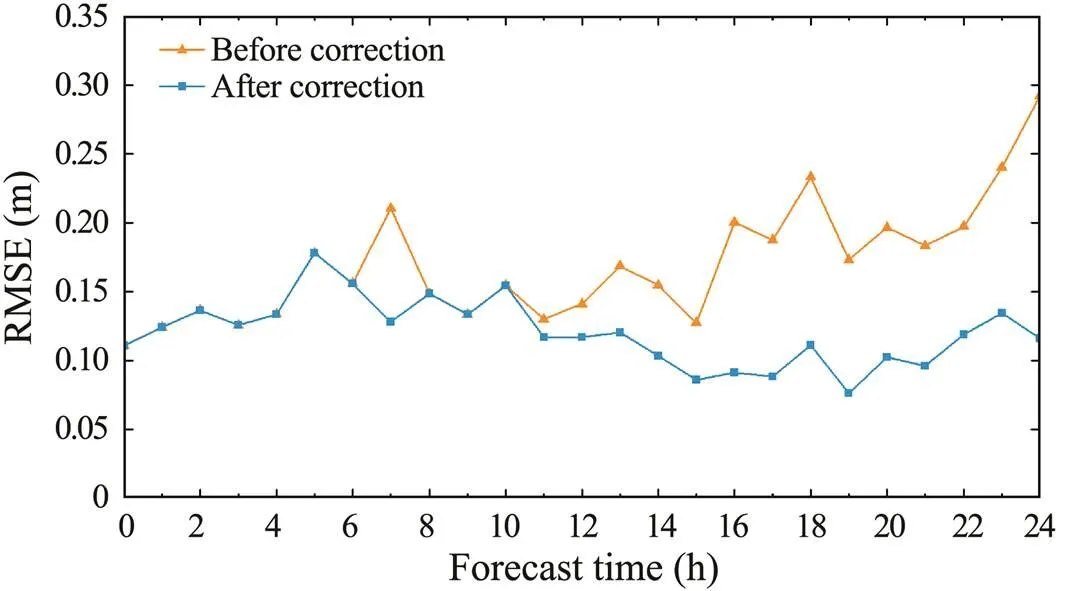
Fig.13 RMSEs of time series prediction correction.
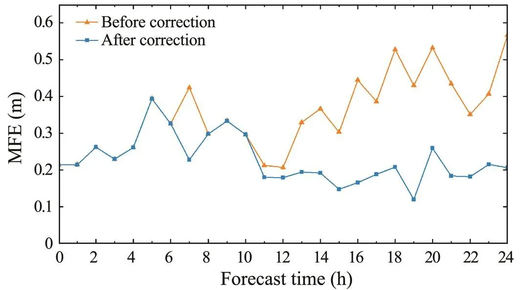
Fig.14 MFEs of time series prediction correction.

Fig.15 Grid point time series.
This method achieves close correspondence between the forecasting results and the manual forecasts obtained by professional knowledge and experience from forecasters to correct the forecasting field data. It can also realize the efficient correction of the bias of the significant wave height numerical model in operational prediction tasks. The forecasting effect of the correlation forecasting time is significantly improvedthe analysis and correction of the numerical forecasting results in spatiotemporal dimensions. The programing language is used to test the efficiency of the time series interpolation. The calculation time, which is influenced by the influence radius of the time series interpolation and the computer performance, is inconsistent, but it can be completed within 10s. Moreover,the correction method of spatial bias for numerical prediction proposed in this paper is easy to operate. The proposed method realizes the linkage correction of time series on the basis of maintaining the temporal development trend of the numerical prediction system, thereby effectively improving the efficiency of prediction correction.
5 Conclusions
This paper proposes a spatiotemporal interactive processing bias correction method for the numerical prediction of significant wave heights based on the operating requirements of ocean wave forecasting by using subjective and objective fusion technology. The method can efficiently correct any gridded point of the spatial field of numerical models by spline interpolation with barriers and sub-zone numerical analysis, which are carried out to address the uncertainty of interpolation results. The SPCF was divided into large and small correction areas for outlier processing and overall trend adjustment, respectively, to ensure the rationality of the spatial interpolation results. The spatial prediction correction results were also interpolated into the whole or its adjacent time series by successive correction analysis to satisfy the requirement of timeliness. After correction, the data transition of the time series became smooth, and the correction process did not affect the overall trend of the forecasting time series in the numerical model.
The correction process and effect of spatiotemporal series were analyzed by using buoy observations; here, the numerical model prediction of significant wave heights from the ECMWF was taken as an example. The experiment showed that the proposed method could achieve effective correction results and, thus, is applicable for the processing of spatiotemporal data in marine wave forecasting. Forecasters can edit the spatial prediction field through rapid human-computer interaction and correct temporal predictions by using the automated algorithm to improve the efficiency of manual correction of numerical prediction bias. The prediction correction algorithm proposed in this paper can be applied to the production and release of operational ocean wave forecasting products to enhance the efficiency of human-computer interactive processing forecasting bias.
This paper mainly conducts research on an interactive correction algorithm based on the spatiotemporal correlation of numerical model predictions and the experience of forecasters. The current algorithm will be improved to refine the level of marine forecasts in future work. Considering the shortcomings of the current correction method for near-shore data, the spatial interpolation algorithm will be further combined with the physical laws of ocean waves to improve its scientific applicability and rationality. Artificial intelligence methods may also be employed to further mine the spatiotemporal nonlinear characteristics of numerical models and achieve the application goal of intelligent grid forecasting. The combination of forecasters’ experience and artificial intelligence methods can compensate for the influence of the uncertainty of numerical forecasting on the accuracy of marine forecasts and improve the ability of the latter.
Acknowledgements
This work was supported by the National Key Research and Development Program of China (No. 2018YFC1407002), the National Natural Science Foundation of China (Nos. 62071279, 41930535), and the SDUST Research Fund (No. 2019TDJH103).
Americal Meteorlogical Society, 2002. Implementation challenges of IFPS at a forecast office with complex terrain. https://ams.confex.com/ams/annual2002/webprogram/Paper27252.html.
Bannister, R. N., Chipilski, H. G., and Martinez-Alvarado, O., 2020. Techniques and challenges in the assimilation of atmospheric water observations for numerical weather prediction towards convective scales., 146 (726): 1-48.
Ben Alaya, M. A., Cheban, F., and Ouarda, T. B. M. J., 2015. Probabilistic multisite statistical downscaling for daily precipitation using a Bernoulli-generalized Pareto multivariate autoregressive model., 28 (6): 2349-2364.
Benjamin, S. O., and Seaman, N. L., 1985. A simple scheme for objective analysis in curved flow., 113 (7): 1184.
Bourgin, F., Ramos, M. H., Thirel, G., and Andreassian, V., 2014. Investigating the interactions between data assimilation and post-processing in hydrological ensemble forecasting., 519: 2775-2784.
Briggs, I. C., 2012. Machine contouring using minimum curvature., 39 (1): 39-48.
Chattopadhyay, A., Nabizadeh, E., and Hassanzadeh, P., 2020. Analog forecasting of extreme-causing weather patterns using deep learning.,12 (2): e2019MS001958, https://doi.org/10.1029/2019MS001958.
Chen, S. H., Yang, S. C., Chen, C. Y., van Dam, C. P., Cooperman, A., Shiu, H.,, 2019. Application of bias corrections to improve hub-height ensemble wind forecasts over the Tehachapi Wind Resource Area., 140: 281-291.
Chu, Y. Q., Li, C. C., Wang, Y. F., Li, J., and Li, J., 2016. A long-term wind speed ensemble forecasting system with weath- er adapted correction., 9 (11): 894, https://doi.org/10.3390/en9110894.
Cui, B., Toth, Z., Zhu, Y., and Hou, D. C., 2011. Bias correctionfor global ensemble forecast., 27 (2): 396-410.
Du, P. J., Wang, L. L., Guan, Q. L., Xue, J. L., Chen, X. E., Kang, X.,, 2013. Development and applications of an interactive operational forecast system on typhoon induced wave., 43 (10): 16-24 (in Chinese with English abstract).
Duan, Q., Di, Z., Quan, J., Wang, C., Gong, W., Gan, Y.,, 2017. Automatic model calibration: A new way to improve numerical weather forecasting., 98 (5): 959-970.
Durai, V. R., and Bhradwaj, R., 2014. Evaluation of statistical bias correction methods for numerical weather prediction model forecasts of maximum and minimum temperatures., 73 (3): 1229-1254.
Epstein, E. S., 1969. Stochastic dynamic prediction., 21 (6): 739-759.
Fei, L., 2018. Spatial interpolation algorithm research of ArcGIS engine.. University of Salford, Man- chester, 97-99.
Gao, S., Dai, K., and Xue, F., 2014. The design and development of grid edit platform based on MICAPS 3.2 system., 40 (9): 1152-1158 (in Chinese with English abstract).
Goyal, M., Panchariya, V., Sharma, A., and Singh, V., 2018. Comparative assessment of SWAT model performance in two distinct catchments under various DEM scenarios of varying resolution, sources and resampling methods., 32 (2): 805-825.
Guan, H., Cui, B., and Zhu, Y. J., 2015. Improvement of statistical postprocessing using GEFS reforecast information., 30 (4): 841-854.
Hart, K. A., Streenburgh, W. J., Onton, D. J., and Siffert, A. J., 2004. An evaluation of mesoscale-model-based model output statistics (MOS) during the 2002 Olympic and Paralympic Winter Games., 19 (2): 200-218.
He, Y. N., Gao, S., Xue, F., Zhao, S. R., Liu, M., Hu, H.,, 2018. Design and implementation of intelligent grid forecasting platform based on MICAPS4., 29 (1): 13-24 (in Chinese with English abstract).
Hu, S. J., Qiu, C. Y., Zhang, L. Y., Huang, Q. C., Yu, H. P., and Chou, J. F., 2014. An approach to estimating and extrapolating model error based on inverse problem methods: Towards accurate numerical weather prediction., 23 (8): 89201.
Irmak, A., Ranade, P. K., Marx, D., Irmak, S., Hubbard, K. G., Meyer, G. E.,, 2010. Spatial interpolation of climate variables in Nebraska., 53 (6): 1759-1771.
Jin, R. H., Dai, K., Zhao, R. X., Cao, Y., Xue, F., Liu, C. H.,, 2019. Progress and challenge of seamless fine gridded weather forecasting technology in China., 45 (4): 445-457 (in Chinese with English abstract).
Krishnamurti, T. N., Sanjay, J., Mitra, A. K., and Vijay Kumar, T. S. V., 2004. Determination of forecast errors arising from different components of model physics and dynamics., 132 (11): 2570-2594.
Leith, C. E., 1974. Theoretical skill of Monte Carlo forecasts., 102 (6): 409, DOI: 10.1175/1520-0493(1974)102<0409:TSOMCF>2.0.CO;2.
Li, P. C., and Liu, X. D., 2018. Bilinear interpolation method for quantum images based on quantum Fourier transform., 16: 1850031, DOI: 10.1142/S0219749918500314.
Li, Z. X., He, Y. Q., Xin, H. J., Wang, C. F., Jia, W. X., Zhang, W.,, 2010. Spatio-temporal variations of temperature and precipitation in Mts. Hengduan Region during 1960–2008., 65 (5): 563-579.
Liu, G. L., Chen, B. Y., Wang, L. P., Zhang, S. F., Zhang, K. Y., and Lei, X., 2019. Wave height statistical characteristic analysis., 37 (2): 448-460.
Liu, Z. H., Huang, R. G., Hu, Y. M., Fan, S. D., and Feng, P. H., 2011. Generating high spatiotemporal resolution LAI based on MODIS/GF-1 data and combined Kriging-Cressman interpolation., 9 (5): 120-131.
Mass, C. F., 2003. IFPS and the future of the national weather service., 18 (1): 75-79.
Mass, C. F., Ovens, D., Westrick, K., and Colle, B., 2002. Does increasing horizontal resolution produce more skillful forecasts?, 83 (3): 407-430.
Pan, B. X., Hsu, K., AghaKouchak, A., and Sorooshian, S., 2019. Improving precipitation estimation using convolutional neural network., 55 (3): 2301-2321.
Rukundo, O., and Schmidt, S. E., 2018. Effects of rescaling bilinear interpolant on image interpolation quality., 10817: 11-12.
Schulze, G. C., 2007. Atmospheric observations and numerical weather prediction., 103: 318-323.
Smith, W. H. F., and Wessel, P., 1990. Gridding with continuous curvature splines in tension., 55 (3): 293-305.
Susanto, F., de Souza, P., and He, J., 2016. Spatiotemporal interpolationforenvironmentalmodelling.,16:1245,https://doi.org/10.3390/s16081245.
Tang, B. H., and Bassill, N. P., 2018. Point downscaling of surface wind speed for forecast applications., 57 (3): 659-674.
Terzopoulos, D., 1988. The computation of visible-surface representations., 10 (4): 417-438.
Wang, H., Liu, N., Li, B. X., and Li, X., 2014. An overview of ocean predictability and ocean ensemble forecast., 29 (11): 1212-1225.
Wang, T. W., Gao, S., Xu, J. L., Li, Y. R., Li, P., and Ren, P., 2018. Correcting predictions from oceanic maritime numerical modelsresidual learning.. Kobe, Japan.
World Meteorological Organization (WMO), 2015. Seamless pre- diction of the earth system: From minutes to months. https:// library.wmo.int/index.php?lvl=notice_display&id=17276#.XzPlq_kzaUk.
Wu, W., Wu, Z. M., Gao, S. H., and Zheng, Y., 2013. A homogeneous linear estimation method for system error in data assimilation., 12 (3): 335-344.
Yang, S. B., Xia, T. L., Zhang, Z. Q., Zheng, C. W., Li, X. F., Li, H. Y.,, 2019a. Prediction of significant wave heights based on CS-BP model in the South China Sea., 7: 147490-147500.
Yang, S. B., Zhang, Z. Q., Fan, L. L., Xia, T. L., Duan, S. H., Zheng, C. W.,, 2019b. Long-term prediction of significant wave height based on SARIMA model in the South China Sea and adjacent waters., 7: 88082-88092.
Yu, Z. C., Zhong, S. B., Wang, C. L., Yang, Y. S., Yao, G. N., and Huang, Q. Y., 2017. Mapping comparison and meteorological correlation analysis of the air quality index in mid-eastern China., 6 (2): 52, https://doi.org/10.3390/ijgi6020052.
Zhang, H. L., and Pu, Z. X., 2010. Beating the uncertainties: Ensemble forecasting and ensemble-based data assimilation in modern numerical weather prediction., 2010: 432160, DOI: 10.1155/2010/432160
Zhang, H. R., Lu, L. J., Liu, Y. H., and Liu, W., 2015. Spatial sampling strategies for the effect of interpolation accuracy., 4 (4): 2742-2768.
Zoraster, S., 2003. A surface modeling algorithm designed for speed and ease of use with all petroleum industry data., 29 (9): 1175-1182.
November 9, 2020;
January 5, 2021;
May 10, 2021
© Ocean University of China, Science Press and Springer-Verlag GmbH Germany 2022
. E-mail: guojingtian@ncs.mnr.gov.cn
(Edited by Xie Jun)
 Journal of Ocean University of China2022年2期
- Journal of Ocean University of China的其它文章
- Study of the Wind Conditions in the South China Sea and Its Adjacent Sea Area
- Characteristics Analysis and Risk Assessment of Extreme Water Levels Based on 60-Year Observation Data in Xiamen, China
- Underwater Target Detection Based on Reinforcement Learning and Ant Colony Optimization
- Polar Sea Ice Identification and Classification Based on HY-2A/SCAT Data
- Thermo-Rheological Structure and Passive Continental Margin Rifting in the Qiongdongnan Basin,South China Sea, China
- Effect of Penetration Rates on the Piezocone Penetration Test in the Yellow River Delta Silt