
Polar Sea Ice Identification and Classification Based on HY-2A/SCAT Data
2022-02-24 08:10XURuiZHAOChaofangZHAIXiaochunZHAOKeSHENJichangandCHENGe
XU Rui, ZHAO Chaofang, 2), *, ZHAI Xiaochun, ZHAO Ke, SHEN Jichang, and CHEN Ge, 2)
Polar Sea Ice Identification and Classification Based on HY-2A/SCAT Data
XU Rui1), ZHAO Chaofang1), 2), *, ZHAI Xiaochun3), ZHAO Ke1), SHEN Jichang1), and CHEN Ge1), 2)
1),,266100,2),,266100,3),100081,
In this paper, a Bayesian sea ice detection algorithm is first used based on the HY-2A/SCAT data, and a backpropagation (BP) neural network is used to classify the Arctic sea ice type. During the implementation of the Bayesian sea ice detection algorithm, linear sea ice model parameters and the backscatter variance suitable for HY-2A/SCAT were proposed. The sea ice extent obtained by the Bayesian sea ice detection algorithm was projected on a 12.5km grid sea ice map and validated by the Advanced Microwave Scanning Radiometer 2 (AMSR2) 15% sea ice concentration data. The sea ice extent obtained by the Bayesian sea ice detection algorithm was found to be in good agreement with that of the AMSR2 during the ice growth season. Meanwhile, the Bayesian sea ice detection algorithm gave a wider ice edge than the AMSR2 during the ice melting season. For the sea ice type classification, the BP neural network was used to classify the Arctic sea ice type (multi-year and first-year ice) from January to May and October to December in 2014. Comparison results between the HY-2A/SCAT sea ice type and Equal-Area Scalable Earth Grid (EASE-Grid) sea ice age data showed that the HY-2A/SCAT multi-year ice extent variation had the same trend as the EASE-Grid data. Classification errors, defined as the ratio of the mismatched sea ice type points between HY-2A/SCAT and EASE-Grid to the total sea ice points, were less than 12%, and the average classification error was 8.6% for the study period, which indicated that the BP neural network classification was a feasible algorithm for HY-2A/SCAT sea ice type classification.
sea ice; HY-2A/SCAT; sea ice identification; sea ice type; Bayesian sea ice detection; BP neural network
1 Introduction
Sea ice, a sensitive climate indicator, plays several roles in the global climate system and affects the exchange of heat, mass, momentum, and chemical constituents among the ocean, atmosphere, and surface albedo to reduce the amount of solar radiation absorbed at the Earth’s surface. Further, it directly affects ships and offshore operations at high latitudes (Sandven., 2006). In addition, differentsea ice types have distinct physical characteristics, and themulti-year ice has greater thickness and higher albedo than the first-year ice. Thus, the study of both the polar sea ice extent and ice type is of great significance for monitoring global climate changes and fishing situations (Li., 2016).
Sea ice observation methods include ship and aircraft detection, which are not only inefficient and costly but also provide a difficult direct observation of the polar sea ice due to complex geography and unstable climate. With the development of remote sensing technology, the satellite has become an effective means to study the polar sea ice. Visible and near-infrared sensors such as the Advanced Very High Resolution Radiometer (AVHRR) and the Mo- derate Resolution Imaging Spectroradiometer (MODIS) col-lect remote sensing parameters at various wavebands, which have been widely used for sea ice studies (Scott, 2013; Chi., 2019).
However, visible and near-infrared sensors are easily affected by clouds or fog, resulting in fuzzy remote sensing images. Fortunately, microwave sensors became important tools for sea ice observation because of their ability to penetrate clouds and ability to work all day. Microwave radiometers such as the Electrically Scanning Microwave Radiometer (Nimbus-5/ESMR) and the Scanning Multichannel Microwave Radiometer (Nimbus-7/SMMR) can derive the ice extent and ice types by measuring the bright- nesstemperature. Since 1987, Defense Meteorological Sa- tellite Program satellites have been equipped with the Special Sensor Microwave/Imager (SSM/I) and the Special Sensor Microwave Imager/Sounder (SSMIS), which have provided global sea ice information from 1987 to the present. The Advanced Multichannel Scanning Radiometer- EOS (AMSR-E) aboard the EOS-Aqua satellite has a high- er spatial resolution and a larger spectral range than the SSM/I (Nishio and Comiso, 2005). Researches have shown that satellite passive microwave radiometers can be used to estimate both the sea ice concentration and sea ice type over a large space range (Nishio, 2004; Nakata, 2019).
Active microwave sensors for sea ice monitoring primarily include synthetic aperture radar (SAR) and scatte- rometers. In 1978, Seasat-A became the first satellite to pro- vide sea ice high-resolution SAR images. SAR has many unique advantages in sea ice observation, such as the abi- lity to image at a high resolution. However, SAR has a small swath and high data costs, so it is difficult to study the polar sea ice and ocean phenomena of large-scale or mesoscale using the SAR data. Since the 1990s, the microwave scatterometer has been used for sea ice detection, including the Europe Remote Sensing Satellite Scattero- meter (ERS scatterometer) (Otosaka., 2018), the Advanced Scatterometer (ASCAT) at C-band, and the NASA Scatterometer (NSCAT), QUIKSCAT/SeaWinds, HY-2AScatterometer (HY-2A/SCAT) at the Ku-band. Even thoughthe microwave scatterometer was originally designed to retrieve wind fields by measuring the backscattering coefficient (0), with the deepening understanding of the microwave scattering of sea ice, microwave scatterometer data has become more and more mature in sea ice detection in recent years (Long, 2017; Zhang, 2019; Bi, 2020).
For sea ice identification, two main sea ice detection algorithms based on the Ku-band microwave scatterometer were proposed: 1) the Remund and Long-NSCAT Algorithm (RL-N algorithm) (Remund and Long, 1997) and 2) the Bayesian sea ice detection algorithm (Rivas and Stof- felen, 2011). In 1997, Remund and Long developed an au- tomatic algorithm for sea ice and open water discrimination based on the Ku-band NASA Scatterometer (NSCAT) data and validated it by comparing the sea ice extent result with SSM/I sea ice concentration datasets (Remund and Long, 1997, 1999). Later, the algorithm was modified to apply for the QUIKSCAT/SeaWinds and to release the QUIKSCAT and Oceansat-2 Scatterometer (OSCAT) BUFR (the binary universal form of the representation of meteorological data) geophysical products. The RL-N algorithm for the QUIKSCAT/SeaWinds uses the maximum likelihood method with a combined matrix [54/46,46, ∆46, ∆54] (horizontal polarization46, polarization ratio54/46, dual-polarization standard deviation ∆46and ∆54) acting as discriminant parameters to detect sea ice. The residual error due to high-persistent winds over the sea surface is solved by sea ice growth/retreat constraint methods (Remund and Long, 2014).
The Bayesian sea ice detection algorithm, combining both wind and sea ice maximum likelihood estimators withprior information to discriminate sea ice, was first employ- ed by the C-band microwave scatterometer (Haan and Stof-felen, 2001). The sea ice edge of the C-band ASCAT based on the Bayesian sea ice detection algorithm is in good agreement with the sea ice edge defined by the AMSR-E 15% concentration isoline in winter (Rivas, 2012). In 2009, this algorithm was applied to the Ku-band QUIKSCAT/SeaWinds, and an additional sea surface temperature (SST) filter was added to reduce the error caused by occasional erratic winds over the sea ice surface (Rivas and Stoffelen, 2009).
In addition to sea ice identification, the microwave scatterometer has also been used to classify the sea ice type. Sea ice can be classified into new ice, Nilas ice, young ice, first-year ice (FYI), and multi-year ice (MYI) based on the growth process.
It is difficult to distinguish relatively thin ice such as new ice, Nilas ice, young ice with only the backscatter data (Tonboe and Toudal, 2005; Brath, 2013), and there is almost no MYI in the Antarctic due to geographical factors (Tucker, 1992). In this study, sea ice classification is conducted in the Arctic, and only the FYI and MYI are classified. MYI has lower surface salinity and more air voids than FYI since MYI has undergone multiple brine drainages (Tucker, 1992). Since the Ku-band scatterometer is sensitive to volume scattering and air voidsin MYI enhance volume scattering, the backscatter of MYI is characterized by stronger volume scattering than FYI, and MYI appears brighter in the Ku-band microwave scattering image.
Based on the scattering differences mentioned above, many studies on the sea ice type classification using Ku- band microwave scatterometers have emerged. Swan and Long (2012) used a time-dependent threshold to classify MYI and FYI based on the QUIKSCAT data from 2003 to 2009. Lindell and Long (2016b) corrected misclassifications in the marginal ice zone (MIZ) caused by the incursion of ocean waves and swells and extended Arctic ice type data records to 2014 using the OSCAT data. For C-band scatterometers, Lindell and Long (2016a) deve- loped a Bayesian estimator to classify the Arctic sea ice using the ASCAT and SSMIS data. The result of the MYI extent is generally consistent with that of the Ku-band OSCAT. Otosaka(2018) proposed a new C-band sea ice backscatter normalization scheme, which is more accurate in the determination of sea ice backscatter modes than existing linear correction approaches. The development of this scheme will consolidate scatterometer capabilities to further investigate sea ice types.
In 2011, the first Chinese marine dynamic environmentalsatellite, HY-2A, was successfully launched. The scattero- meter equipped with the HY-2A (hereafter, HY-2A/SCAT) has been used in many aspects of meteorological research, but sea ice studies based on the HY-2A/SCAT need to be explored further.
In terms of sea ice identification, Zou(2016) used a fixed value of active polarization ratio to achieve preliminary Antarctic sea ice identification based on the HY- 2A/SCAT backscattering coefficient. Compared with sea ice products of the AMSR2, sea ice determination results obtained by this algorithm are in good agreement with those of the AMSR2 in the sea ice development trend, seasonal change, area distribution, and sea ice edge distribution. Li(2016) performed a Fisher linear discri- minant algorithm in the sea ice detection on the polar region based on the HY-2A/SCAT data using the same combined parameter matrix as the RL-N algorithm. Results showed that the HY-2A/SCAT data had good sea ice detection capability.
In terms of sea ice type classification, Li(2016) used the HY-2A/SCAT vertical polarization backscattering coefficient to fit the dynamic classification threshold between MYI and FYI and obtained an Arctic sea ice type over January to May and October to December from 2013 to 2015, which was almost consistent with the ASCAT/ SSMIS sea ice type product.
Overall, for sea ice identification, only the sea ice detection parameters from the RL-N were employed to the HY-2A/SCAT (Li, 2016), while the Bayesian sea ice detection algorithm can better detect thin ice in winter and has less misclassification noise than the RL-N algorithm (Rivas and Stoffelen, 2011). As for the sea ice type classification, there is no other algorithm applied by the Ku-band scatterometer except the dynamic threshold classification algorithm (Swan and Long, 2012; Li, 2016;Lindell and Long, 2016b). Thus, sea ice researches on the HY-2A/SCAT still need supplementation to give us a better understanding of the role of scatterometers in sea ice monitoring.
Therefore, this study applied a Bayesian sea ice detection algorithm, and a preliminary comparison was made between HY-2A/SCAT sea ice discrimination results and those of AMSR2 datasets to validate the feasibility of this algorithm on the HY-2A/SCAT. Moreover, four parameters [fore,fore,aft,aft] were all found to be sensitive to the sea ice type. Considering that the backscattering thres- hold between MYI and FYI varies over time, this work also used the time factor as an important feature of sea ice type classification. To integrate these characteristic parameters into the sea ice type classification, a backpropagation (BP) neural network was employed in this study, which can solve complex internal mechanism problems (Li, 2012). Moreover, the Equal-Area Scalable Earth Grid (EASE-Grid) sea ice age data was employed to validate the sea ice type results. The rest of this article is organized as follows. Section 2 introduces the datasets used in this paper and describes the algorithms used for sea ice identification and sea ice type classification, which are the Baye- sian sea ice detection algorithm and BP neural network, respectively. Results and the validation work are presentedin Section 3. Finally, Section 4 summarizes the results and concludes with notes on future work.
2 Data and Methods
2.1 Datasets
2.1.1 HY-2A/SCAT data used in the study
The scatterometer aboard the HY-2A satellite (HY-2A/ SCAT) is a rotating pencil beam radar with a 13.25GHz operating frequency. The HY-2A/SCAT employs a one-me- ter dish reflective antenna, including two beams, in which the inner beam collects the horizontally polarized (H-pol) backscattering coefficient at an incidence angle of 41˚ (41), and the outer beam collects vertically polarized backscattering coefficient at incidence angle of 48˚ (48). Therefore, each surface observation cell is viewed four times, forward and afterward looking by the inner (fore,aft) and outer beam (fore,aft), respectively (Wang, 2012). These four parameters are used in accomplishing the Bayesian sea ice detection algorithm and the BP neural network sea ice type classification. Fig.1 shows the scatterometer observation geometry.
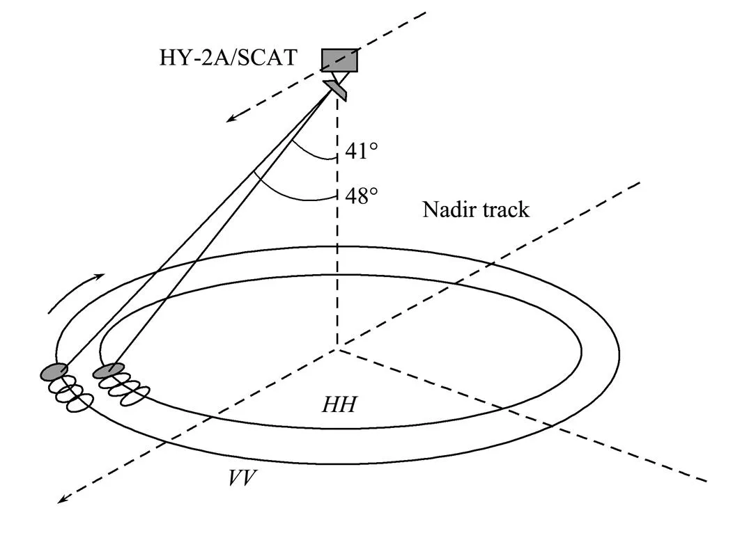
Fig.1 Scatterometer observation geometry (Wang et al., 2012). Incidence angles for the inner HH and outer VV polarized beams are 41˚ and 48˚, respectively.
HY-2A/SCAT L2A data from both Arctic and Antarctic regions were used for the study.
According to Zhao and Zhao (2019), the wind speed root mean square error between the HY-2A/SCAT and buoys from 2012 to 2018 is lowest in 2014. Therefore, HY/SCAT data from 2014 was used to explore how sea ice monitoring algorithms could be applied to the HY-2A/SCAT. Figs.2 and 3 show variations of the backscattering coefficient (or normalized radar cross section, NRCS) of an MYI pixel and an FYI pixel in 2013 and 2014, respectively. Similar seasonal variation trends of the MYI backscattering coefficient and the FYI backscattering coefficient can be observed over 2013 and 2014, making it possible to classify sea ice types of 2014 by training data in 2013.

Fig.2 Variation of the backscattering coefficient value of an MYI pixel from 2013 to 2014.

Fig.3 Variation of the backscattering coefficient value of an FYI pixel from 2013 to 2014.
Therefore, the temporal range of the HY-2A/SCAT L2Adata used in this study is from January 1, 2013 to December 31, 2014, in which a one-year data (01/01/2013–12/ 31/2013) was used to train the BP neural network model and data from January 1, 2014 to December 31, 2014 was used for the sea ice identification and BP neural network tests.
2.1.2 AMSR2 sea ice concentration data
The AMSR2 unified level-3 sea ice concentration data from January 1, 2014to December 31, 2014 was employ- ed to validate the sea ice identification result. This sea ice concentration data with 12.5km resolution is generated using the enhanced NASA Team (NT2) algorithm (Markus and Cavalieri, 2000, 2009), which has been used as the sea ice extent validation data by other studies (Zou, 2016). The AMSR-E 15% ice concentration isoline has been validated against the MODIS and RADARSAT imagery as a good estimator of the sea ice edge (Heinrichs, 2006). As a replacement for the AMSR-E, the AMSR2 also defined the 15% ice concentration isoline as its sea ice edge.
The daily sea ice concentration data of the AMSR2 can be downloaded from: https://nsidc.org/data/AU_SI12/versions/1(Meier, 2018).
The AMSR2 data applies the National Snow and Ice Data Center (NSIDC) polar stereographic projection, which specifies a projection plane to the Earth’s surface at 70 degrees northern and southern latitude (Snyder, 1987; Pear- son, 1990). For comparison with the AMSR2 sea ice concentration data, HY-2A/SCAT daily0measurements of the polar region are performed on the same projection and resampled into 12.5km resolution (608×896 grid for the Arctic and 632×664 grid for the Antarctic). Fig.4 shows the polar spatial coverage maps.
2.1.3 Numerical weather prediction (NWP) model wind field data
The NWP model wind field data used in this paper was obtained from the European Centre for Medium-Range Weather Forecasts (ECMWF) ERA5 model, which is the fifth generation ECMWF reanalysis for the global climate and weather for the past 4 to 7 decades. The ERA5 wind data is derived by combining the model data and observed data from all over the world based on data assimilation. The NWP model data has become a commonly used reference data in scatterometer wind research since the 1990s(Wentz and Smith, 1999; Bhowmick, 2019). In addition, its wind quality, scatterometer wind quality, and moored buoy wind quality have been commonly assessed through triple collocation (Vogelzang, 2011).
This paper utilized NWP model wind field products from January 1, 2014 to December 31, 2014 to solve the pro- blem of ice and water scattering signal confusion caused by high winds. In addition, the formation of a freshwater surface layer near the ice edge during the ice melting period can change wind geophysical model function (GMF) conditions and result in wind retrieval errors.

Fig.4 Polar spatial coverage maps. (a), Arctic polar stereographic projection region with 12.5km resolution covers 608×896 grids; (b), Antarctic polar stereographic projection region with 12.5km resolution covers 632×664 grids.
The NWP model wind field can help reduce such errors. The ERA5 wind field data can be downloaded from: http://cds.climate.copernicus.eu/cdsapp#!/dataset/reanalysis-era5-single-levels?tab=form.
2.1.4 EASE-Grid sea ice age data
The EASE-Grid ice age data provides weekly estimates of the sea ice age for the Arctic Ocean derived from the re- motely sensed sea ice motion and sea ice extent (Tschudi, 2019). As a remote sensing-based ice age product, it has greater spatial details than the traditional buoy-de- rived age data.
Since the EASE-Grid ice age data can provide a uniform spatial and temporal coverage of the sea ice age product, it is used to model the BP neural network and validate the sea ice type classification result in this study. Note that 16 sea ice ages are included in each EASE-Grid ice type map, in which first-year ice are grouped as FYI, while second-year ice and above are grouped as MYI.
Different from the polar stereographic projection used for the AMSR2 sea ice concentration data, the EASE-Grid age data adopts a polar aspect azimuthal equal-area projection for the Arctic (Brodzik and Knowles, 2002). Be- fore sea ice type classification, the HY-2A/SCAT L2A data were re-sampled into 12.5km resolution (722×722 grid) using the same projection. The re-sampling was achieved based on the EASE-Grid map projection definitions (https://nsidc.org/ease/ease-grid-projection-gt). Fig.5 shows the EASE-Grid sea ice age image and the HY-2A/SCAT Arctic horizontally polarized backscattering coefficient () image after reconstruction. The EASE-Grid sea ice age data spatial range used in the study lies between 29.7˚N to 90˚N latitude and from 180˚W to 180˚E longitude. The temporal range is from 2013 to 2014.

Fig.5 EASE-Grid sea ice age image and HY-2A/SCAT H-pol backscattering coefficient image after interpolation. (a), EASE- Grid sea ice age data in the 1st week of 2014; (b), HY-2A/SCAT σH data on January 2, 2014.
2.2 Sea Ice Identification
In this study, sea ice identification is based on the com- bination of the maximum likelihood estimator and prior information using the Bayesian equation,., the Bayesiansea ice identification algorithm is adopted. This work used the Pencil Beam Wind Processor provided by the Royal Netherlands Meteorological Institute (KNMI) (https://nwp-saf.eumetsat.int/site/software/scatterometer/penwp/) to con-duct the Bayesian sea ice detection algorithm. Since theestablishment of wind and ice GMFs is an essential step of the Bayesian sea ice identification algorithm, GMFs used in this study are first described.
2.2.1 Geophysical model functions (GMFs)
GMFs are empirical functions describing the relationship between backscatter measurements and surface conditions observed from various incidence and azimuth angles. For a given observation geometry, the backscatter from theocean surface is mainly determined by wind speeds and di- rections. Therefore, a wind GMF can well explain the scat- tering characteristics of the ocean surface. The Ku-band wind GMF is established based on the comparison between NSCAT backscatter measurements and ECMWF NWP wind field (Wentz and Smith, 1999). The wind GMF for the Ku-band can be downloaded from https://scatte- rometer.knmi.nl/nscat_gmf/.
The empirical GMF for sea ice was derived based on the observed backscattering coefficient distribution of pure sea ice (100% concentration) in winter and was found to be a linear distribution in the Ku-band scatterometer four- dimensional observation space (fore,aft,fore,aft) (Rivas and Stoffelen, 2009). Fig.6 shows the observed backscattering coefficient distribution of pure sea ice in the HY- 2A/SCAT measurement space. Since scattering from the sea ice is azimuthal isotropic at the Ku-band (.,fore=aftandfore=aft), Fig.6 can represent the distribution of the sea ice backscattering coefficient for both ‘fore’ and ‘aft’ measurement subspaces.andbackscatter components always maintain a fixed ratio (the slope of the line in Fig.6) no matter how the seasons change (Rivas and Stoffelen, 2011). However, this fixed ratio may vary for different scatterometers due to differences in the observation geometry between scatterometers, such as the difference in incidence angles. A fixed ratio of 1.09 was obtained by averaging the fitting slopes ofandbackscatter components of pure sea ice in the Arctic winter of 2014 with an offset of −0.49 (fore=1.09×fore−0.49 oraft=1.09×aft−0.49 for sea ice).

Fig.6 HY-2A/SCAT sea ice model in the HY-2A/SCAT measurement space. Gray points indicate backscattering co- efficients corresponding to pure sea ice, and the straight line corresponds to the ice model line.
2.2.2 Maximum likelihood estimator (MLE)
After the GMF is established, the normalized maximum likelihood estimator can be calculated to the GMF as follows (Rivas and Stoffelen, 2009):


The variability of the sea ice backscattering coefficient (var[0 ice,]) can be derived from the distribution of pure sea ice backscatter distances to the linear sea ice GMF (Rivas and Stoffelen, 2009), in which the distribution is Gaussian. Fig.7 shows the schematic diagram of the sea ice backscattering coefficient distance to the linear ice model. A is a random sample point, and the distance is the vertical distance from A to the linear ice model. Since sea ice scattering is azimuthal isotropic in the Ku-band, this distance can be determined using allandbackscatter components, whether obtained from the ‘fore’ view or from the ‘aft’ view.
Fig.8 shows the distribution of the distance for the Arctic on March 21, 2014, and the Antarctic on September 21, 2014. The distance distribution was fitted for each day in 2014, and the daily Gaussian fitting standard deviation valuewas obtained, as shown in Fig.9. Assuming that the Gaussian standard deviation is expressed as STDEV. var[0 ice,] is then defined as {Mean[(Arctic winter,Antarctic winter)]}2, in whichArctic winter andAntarctic winter indicate the averagein Arctic and Antarctic winters, respectively. The average of these two was taken as the final standard deviation, which is 0.4dB. The mean value was used to ensure that this variance will not be too large for any polar region in this study. Then, the var[0 ice,] is the square of the final standard deviation.
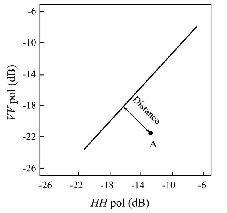
Fig.7 Schematic diagram of the sea ice backscattering coef- ficient distance to the linear ice model. A is a random sample point, and the distance is the vertical distance from A to the linear ice model.
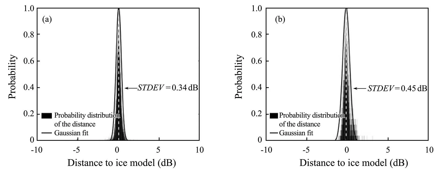
Fig.8 Distribution of the distance between the sea ice backscattering coefficient and the ice model (a)for the Arctic on March 21, 2014, and (b) for the Antarctic on September 21, 2014.

Fig.9 Daily Gaussian fitting standard deviations in 2014 for the Arctic (a) and for the Antarctic (b). The dashed line represents the winter period.
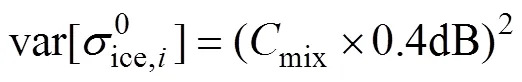
However, lower sea ice fractions during the summer months and those along the Antarctic sea ice margin all year round can increase the variance. Therefore, it is necessary to introduce a tolerance factormixto solve the pro-blem of a larger backscatter variance exhibited by lower sea ice fractions (Rivas and Stoffelen, 2011). Finally, var[0 ice,] can be defined as:
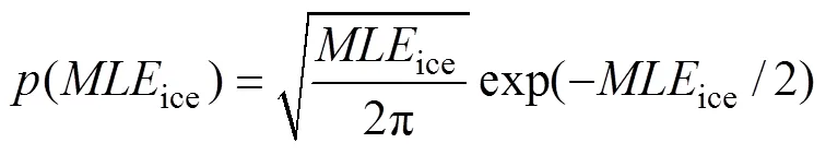
Since theiceandwindare expressed as the sum of four squared standard Gaussian variables for the HY-2A/SCAT, probabilities(wind) and(ice) can be mo- deled as chi-square functions with 2(−2) and 3(−1) de- grees of freedom (Rivas and Stoffelen, 2011):

2.2.3 Bayesian formula
The last step of the Bayesian sea ice detection algorithm is to compute the posterior probability, which can be obtained by combining prior probabilities (0(ice),0(wind))with the expected distribution of theusing the Baye- sian equation:

where the conditional probability(0|wind) and(0|ice)are defined as(wind) and(ice) respectively men-tioned in the previous section:
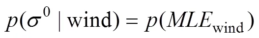

However, the backscatter of MYI is similar to that of the high wind, which may confuse the MYI scattering signal with that of the seawater. To solve this problem, a prior constraint based on the NWP model windNWPfrom the ECMWF is employed. Then,(0|wind) is ultimately defined as:

where ∆is the standard deviation of retrieved wind solutions about the NWP model wind. ∆is set to be 5 in this study.is the apparent surface wind velocity derived from the HY-2A/SCAT.
The prior sea ice probability0(ice) and wind probabi- lity0(wind) are initialized to 0.5. To make full use of prior historical information,0(ice) and0(wind) are updated every orbit as0(ice)=(ice|0) and0(wind)=1−0(ice) using the posterior probability of previous pass posteriors in Eq. (6). The updated principle used by SeaWinds has been found to maximize the quality of the prior information and is efficient at inhibiting rain contamination. Hence, the same setting was applied in this study, which is as follows:
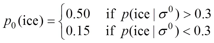
Finally, the sea ice extent was determined using the same threshold (0.55) to the posterior probability in Eq. (6) as the QUIKSCAT (Rivas and Stoffelen, 2009).
2.3 Sea Ice Type Classification
2.3.1 Parameters used in sea ice type classification
Previous studies for sea ice type classification for a Ku- band scatterometer mainly used the V-pol backscattering coefficient () (Swan and Long, 2012; Li, 2016; Lindell and Long, 2016b). In fact, the forward H-pol backscattering coefficient (fore), forward V-pol backscat- tering coefficient (fore), backward H-pol backscattering coefficient (aft), and the backward V-pol backscattering coefficient (aft) all show sensitivities to different ice types.Although theandbackscatter components of pure sea ice in winter are linearly distributed, lower sea ice fractions can increase the dispersion of the distribution. Therefore, bothandbackscatter components were applied to classify the sea ice type instead of using only.
Figs.10a–d shows the distribution histogram of obser- ved values in terms offore,fore,aft, andaftover the Arc-tic sea ice in 2014. These parameters were regularized from −25dB to −5dB at an interval of 0.2. The color in Fig.10 represents the number of different observation va- lues, which were normalized to a range of 0–1. Two distribution peak trends of MYI and FYI can be observed in Figs.10a–d. The trends of these four parameters are rough- ly the same. Variations of MYI and FYI are relatively stable from January to April, and MYI tends to approach the FYI in May with slightly confused scattering signals. MYI and FYI overlap from June to September, making it difficult to distinguish sea ice types. FYI parameters decrease rapidly from October to November and rise slightlyin December. As the temperature rises in summer, ice melt- ing will lead to backscattering confusion between MYI and FYI, making it difficult to distinguish ice types (Li, 2016). Therefore, these four parameters can be used to classify ice types from January to May and October to December.
Besides, the EASE-Grid product provides a weekly sea ice type product. Thus, a weekly average of the above cha- racteristic parameters was made,., the sea ice type obtained in this study is the weekly product.
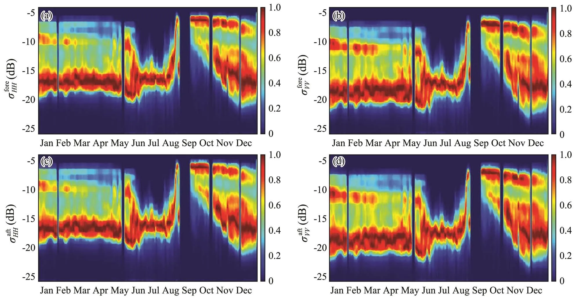
Fig.10 Histogram of the statistical distribution of observed values of different parameters over the Arctic sea ice region in 2014. (a), σfore HH; (b), σfore VV; (c), σaft HH; and (d), σaft VV.
Based on these characteristics, the four weekly-averaged backscattering parameters were used as the input of the BP neural network. Since we found that the threshold between MYI and FYI varies with the season from Fig. 10, this work also added the week number (., 1–52) as the input of the BP neural network. Therefore, five features of [fore,fore,aft,aft,week number]are used as the BP neural work input, and the corresponding output is the ice type flag (FYI, 0; MYI, 1).
2.3.2 Backpropagation (BP) neural network
The backpropagation (BP) neural network is one of the most widely used neural networks that adopt a multi-layer feedforward network based on an error backpropagation algorithm. The BP neural network can learn and store a large number of input-output mode mapping relations with- out revealing the mathematical equations describing the mapping relations in advance (Li, 2012).Note that in the following, this paper will mostly use the abbreviation ‘NN’ to refer to the BP neural network.
In the NN modeling process,samples are randomly divided into training samples and validation samples,in which the training samples are used to train the NN, while the validation samples are used to monitor the NN performance and to find the optimal number of hidden layers by manual adjustment.When the mean squared error of these validation samples reaches its minimum value, the network modeling is considered complete.After NN mo- deling,test samples are used to verify whether the NN re- sults meet experimental requirements.
In this study,data of 35 weeks (containing a total of 1951784 matched cell samples over the sea ice region)in 2013 were used to model the NN,of which 70% of the samples(1366249 matched cell samples)are used for neural network training, and 30%(585535 matched cell samples) were used as validation samples to find the optimal number of hidden layers.After modeling the NN,the data in 2014 were used to test the NN training results that con- tain 1930096 matched samples.
Since a three-layer neural network can approximate any nonlinear function (Goodfellow, 2016), a 5-9-1 NN structure was identified to carry out the sea ice type classification.The number of input layer neurons was determined according to the dimension of the characteristic parameters ([fore,fore,aft,aft, week number]).The number of hidden layer neurons was determined by manual tuning based on the validation samples mentioned above. One neuron in the output layer is used in this study,in which a ‘0’ value of output indicates that the classification result is FYI, while a ‘1’ value indicates that the classification result is MYI. Fig.11 shows the NN structure,where M re- presents the number of hidden layer neurons and Z repre- sents the output.
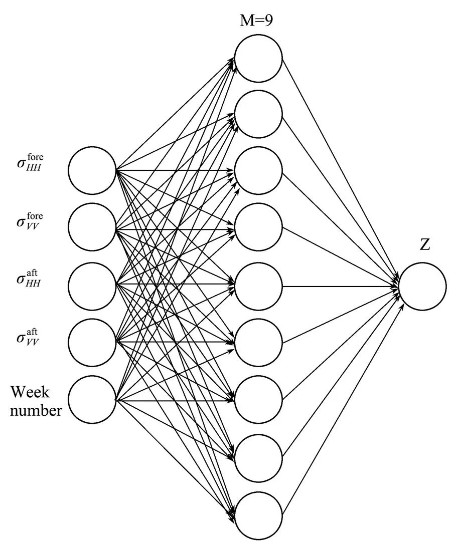
Fig.11 Schematic diagram of the NN structure. The NN structure used in this study consists of three layers, with five neurons in the input layer, nine neurons in the hidden layer, and one neuron in the output layer.
3 Results and Validation
3.1 Sea Ice Identification Results and Validation
Research has shown that the AMSR2 15% ice concentration isoline currently provides the best available representation of the sea ice edge in the ice growth season (fall and winter) but tends to underestimate the sea ice extent during the ice melting season (spring and summer) due to weather effects, unresolved ice types, and surface melt con-ditions (Markus and Cavalieri, 2000). Therefore, this study used the sea ice concentration data of the AMSR2 in the ice growth season to validate the sea ice extent of the HY- 2A/SCAT.
3.1.1 Adjustment of the tolerance factormix
At the beginning of the validation work, the optimal va- lue ofmixwas determined by comparing the sea ice extent of the HY-2A/SCAT with that of the AMSR2 (15% ice concentration isoline) in the ice growth season. Fig.12 shows the AMSR2 sea ice extent and that of the Bayesian sea ice detection algorithm under three tolerance coefficients (mix=1, 2, 3) from January 1, 2014 to December 31, 2014.
Fig.12 Daily sea ice extents of the polar area obtained under three differentCmix values from January 1, 2014 to December 31, 2014. Gray straight lines represent theperiod without HY-2A/SCAT data.
As observed from Fig.12, the total extent of sea ice detected by the scatterometer increases with the increase of the tolerance coefficientmix. Actually, with an increasing value of the tolerance coefficient, the scatterometer can detect more water-saturated ice in the melting season, low concentration ice in the MIZ, and partly translucent ice rapidly formed in the fall (Rivas and Stoffelen, 2011).
To obtain the optimal tolerance coefficient value, this study calculated the absolute difference between the sea ice extent of the HY-2A/SCAT and AMSR2 under different tolerance coefficients, as shown in Fig.13. For the ice growth season in the Arctic, the absolute mean differences between the HY-2A/SCAT sea ice extent and that of the AMSR2 are 0.53×10⁶km2(mix=1), 0.38×10⁶km2(mix=2), and 1.20×10⁶km2(mix=3) for the three tolerance coefficients. For the ice growth season in the Antarctic, the absolute mean differences between the HY-2A/ SCAT sea ice extent and that of the AMSR2 are 0.56×10⁶km2(mix=1), 0.24×10⁶km2(mix=2), and 2.10×10⁶km2(mix=3) for the three tolerance coefficients.
The AMSR2 15% ice concentration isoline provides a reliable sea ice edge in the ice growth season. In addition, the statistics shown in Fig.13 prove that when the tolerance coefficient value is set to 2, the sea ice extent obtained by the HY-2A/SCAT has the smallest deviation from that of the AMSR2 during the ice growth season. Therefore, themixvalue was set to 2.

Fig.13 Sea ice extent absolute differences (×106km2) for the Arctic (a) and the Antarctic (b) between the HY-2A/SCAT and AMSR2 under different tolerance coefficients in 2014.
3.1.2 Sea ice extent obtained by the Bayesian sea ice detection algorithm
After determining the value ofmix, the daily sea ice extent maps in 2014 were obtained using the Bayesian sea ice detection algorithm. Fig.14 shows several maps of the sea ice extent. The Arctic sea ice extent obtained by the Bayesian sea ice detection algorithm is shown in the upper panel, while the lower panel shows the Antarctic sea ice extent. Each panel demonstrates four days’ sea ice extents, in which these four days are selected from four seasons. Table 1 lists the mean sea ice extent for four seasons of the Arctic and Antarctic. The seasonal variation of the sea ice extent can be seen from both the image sequences and Table 1. Both for the Arctic and the Antarctic, the sea ice extent is at its highest in winter and at its lowest in summer. Fall and winter are at the growth seasons of the sea ice, while spring and summer are at the sea ice melting seasons. Note that the Bayesian sea ice detection ice maps of the HY-2B/SCAT are available in: https://scatterometer. knmi.nl/hy2b_25_prod/index.php?cmd=ice_maps&period=week&day=0&flag=yes. Since the HY-2B/SCAT is the continued mission of the HY-2A/SCAT, comparing the sea ice extent products of the HY-2B/SCAT and HY-2A/ SCAT will help us better evaluate the sea ice monitoring capabilities of the HY-2B/SCAT and HY-2A/SCAT. This will be one of the main contents of our future research.

Fig.14 Bayesian sea ice detection sea ice maps from four seasons. The upper panel shows the Arctic ice maps, and the lower panel shows the Antarctic ice maps.

Table 1 Average sea ice extent at different seasons (×106km2)
3.1.3 AMSR2 sea ice concentration data validation
The sea ice extent of the Bayesian sea ice detection algorithm (mix=2) is compared with the AMSR2 ice extent defined by the 15% ice concentration isoline from January 1, 2014 to December 31, 2014 in Fig.15.
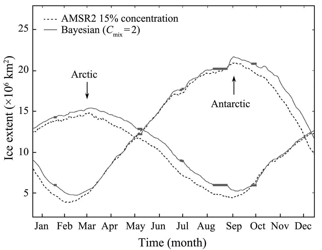
Fig.15 Daily sea ice extents of the polar area of the HY- 2A/SCAT and AMSR2 from January 1, 2014 to December 31, 2014. Gray straight lines represent the period without HY-2A/SCAT data.
From Fig.15, in the sea ice growth season,., the upward branches, the sea ice extent obtained from the HY- 2A/SCAT and AMSR2 is in a high coincidence with absolute mean differences of 0.35×10⁶km2in the Arctic and0.22×106km2in the Antarctic. However, the Bayesian sea ice detection algorithm overestimates the sea ice extent in the ice melting season (downward branches) relative to the AMSR2, with mean differences of 1.21×10⁶km2in the Arctic and 1.22×10⁶km2in the Antarctic.
To further explain the differences between the HY-2A/ SCAT and AMSR2, the AMSR2 15% ice concentration iso- line was used to verify the sea ice edge of the Bayesian sea ice detection algorithm.
Fig.16 shows the ice edge comparison of the Arctic and the Antarctic of June 21, 2014 and December 22, 2014 be- tween the Bayesian sea ice detection and AMSR2, overlaying on the sea ice concentration map of the AMSR2.
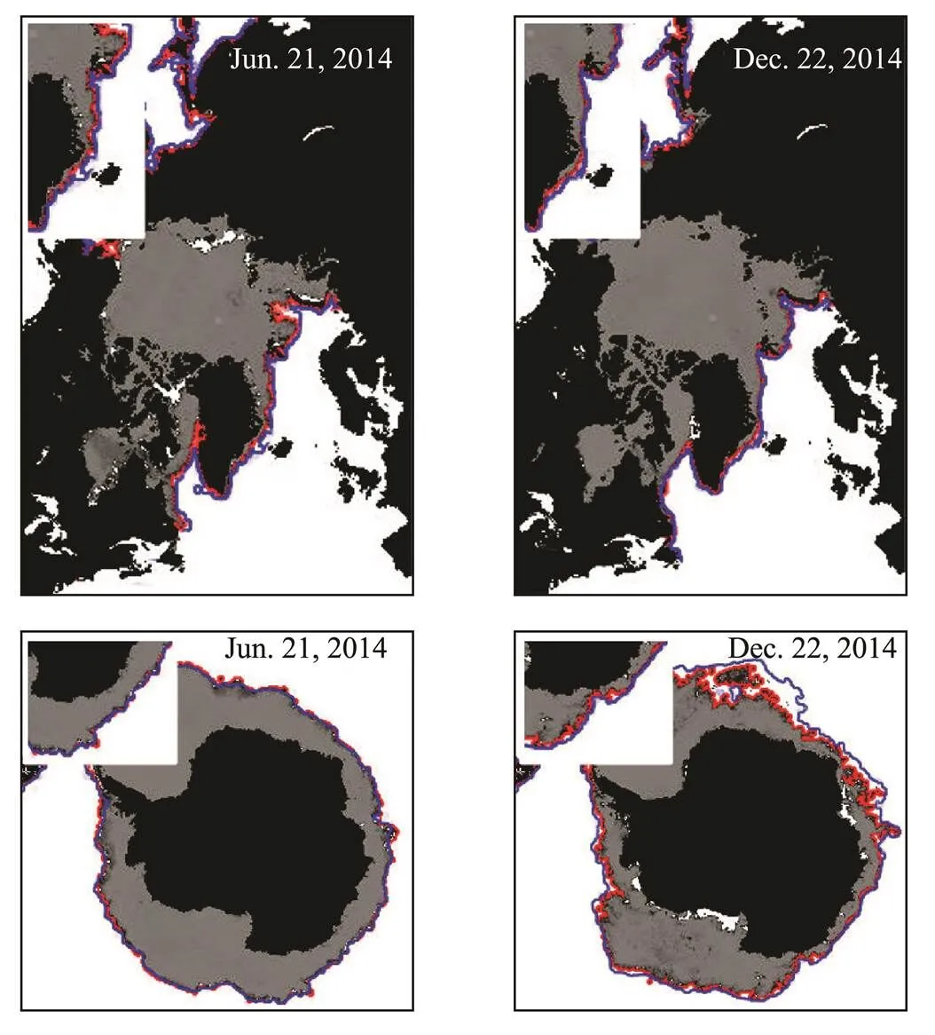
Fig.16 Bayesian sea ice detection algorithm sea ice edge against the AMSR2 15% ice concentration isoline on June 21, 2014 and December 22, 2014. The blue line indicates the Bayesian sea ice detection algorithm sea ice edge and the red line indicates the AMSR2 ice edge.
Ice edges obtained by the Bayesian sea ice detection algorithm and AMSR2 were observed to be very close on June 21, 2014 for the Antarctic and on December 22, 2014 for the Arctic, which means that these two ice edges are very consistent during the sea ice growth season.
The passive microwave algorithm has been proved to be effective in detecting rapidly forming thin ice and provide sea ice edges comparable to those of high-resolution SAR images in the ice growth season (Heinrichs, 2006). Since the ice edges between the Bayesian sea ice detection algorithm and AMSR2 are highly consistent during this period, the Bayesian sea ice detection algorithm can be considered reliable for sea ice detection in the ice growth season.
As for the ice melting season, the ice edge of the Baye- siansea ice detection algorithm was observed to be wider than that of the AMSR2 on December 22, 2014 for the Antarctic, and on June 21, 2014 for the Arctic. When the sea ice is melting, there exist decaying floes with a lower concentration in the sea ice edge. Worby and Comiso (2004) found that the passive microwave radiometer algorithm is likely to ignore the presence of these ice floes, which indicates that the AMSR2 may underestimate the sea ice extent during this period. Rivas and Stoffelen (2011) also proved that the Bayesian sea ice detection algorithm could better detect ice floes than the AMSR-E in the ice melting season by comparing with MODIS and Advanced Synthetic Aperture Radar products. The results of this study were consistent with the results of the Bayesian sea ice detection algorithm on the QUIKSCAT. Therefore, it’s rea- sonable that the HY-2A/SCAT ice edge obtained by the Bayesian sea ice detection algorithm has a wider ice edge than the AMSR2 during the sea ice melting season.
It is worth mentioning that Wang(2017a, 2017b) proposed a new Ku-band wind GMF by evolving the NSCAT-4 based on the sea surface temperature (SST) de- pendence of Ku-band backscatter measurements. Since the sea ice in the MIZ is strongly affected by the SST through lateral heat transport (Ren, 2021), an attempt was made to retrieve the Arctic sea ice extent from the ice growth period and ice melting period using the Ku-band GMF with the SST dependence correction. Results indicated that the Bayesian sea ice detection algorithm with the SST correction produced a slightly lower ice extent than that without SST correction during both the ice growth period and ice melting period. The causes of this pheno- menon were not investigated further because the new GMF with the SST dependence correction hasn’t been widely validated and officially released. However, this issue will be an important part of our future research work because the SST is indeed an important factor for sea ice retrieval.
3.2 Sea Ice Type Classification Results and Validation
3.2.1 Sea ice types obtained by BP neural network
The NN sea ice type classification was carried out from January to May and October to December in 2014, and eight sea ice type images were selected from the eight mon- ths for display, as shown in Fig.17. The dark blue part re- presents the area of the EASE-Grid ice age data for which sea ice types are not calculated. As can be seen from Fig.17, the MYI mainly exists in the Arctic core zone, and a small amount of MYI is also found in the Greenland Sea.
Fig.18 shows the variation of the MYI extent and FYI extent. Note that the total sea ice extent here is defined by the EASE-Grid sea ice age data, which excludes the passages in the Canadian Archipelago. From Fig.18, the change of the FYI extent is relatively large, with a difference of 7.28×10⁶km2from a maximum in March (8.45×10⁶km2) to a minimum in October (1.17×10⁶km2). On the contrary, the variation of the MYI extent was relatively stable, with a difference of 1.69×10⁶km2from a minimum in May (1.35×10⁶km2) to a maximum in October (3.04×10⁶km2). Moreover, the variation of the FYI extent is basically consistent with the variation of the total sea ice extent, which can reflect the seasonal sea ice trend.

Fig.17 Sea ice type images of 8 weeks (2nd week, 6th week, 10th week, 15th week, 19th week, 41st week, 45th week, 50th week).

Fig.18 Time series of the NN MYI extent, NN FYI extent, and EASE-Grid total ice extent. The gray part indicates the period from June to September without NN classification.
3.2.2 EASE-Grid sea ice age data validation
Fig.19 shows the sea ice type map of the EASE-Grid in the 13th week of 2014 on the left and the ice type obtained by the NN on the right. The MYI distribution obtained by NN was observed to be underestimated compared with the EASE-Grid ice type product, which can be confirmed further in Fig.20.
Fig.20 shows trends of the MYI extent from the NN and EASE-Grid. From Fig.20, the EASE-Grid MYI extent was observed to reach its maximum in late September, with an MYI extent of 3.64×10⁶km2. Meanwhile, the NN MYI extent reached its maximum in October, with an MYI extent of 3.04×10⁶km2. From then on, the MYI ex- tent presents a gradual decrease until December. From Jan- uary to May, both MYI extents of the NN and EASE-Grid showed declining trends. Among them, the declining trendof the MYI obtained by the NN is basically consistent with that of the EASE-Grid. The reason for the MYI decline at this stage may be caused by ice melting (Lindell and Long, 2016a). The MYI extent of EASE-Grid surges between September and October, which is largely due to the fact that some of the FYI survived to become MYI in September when the ice melted the most.
To further verify the feasibility of the BP NN in sea ice type classification, the HY-2A/SCAT classification error was calculated based on the EASE-Grid ice age data. For areas covered by ice, the pixels where sea ice types between the HY-2A/SCAT and EASE-Grid are not matching are regarded as misjudgment points. The ratio of misjudgement pixels to the total number of ice pixels is the classification error. Fig.21 shows the sea ice classification error stem diagrams from January to May and October to December in 2014. For the time period studied, the classification errors of sea ice are less than 12%, and the maximum classification error occurs in week 50. The average classification error was about 8.6%. The solid line in Fig.21 represents the proportion of unrecognized second-year ice pixels among all misjudgments. The percentage of unre- cognized second-year ice pixels was above 50% for all weeks, which indicates that the NN sea ice type classification algorithm is weaker in identifying relatively young multi-year ice.
Despite the fact that the BP neural network algorithm would underestimate the second-year ice, the mean classification error of 8.6% proves that the BP neural network has a good mapping ability to learn the mapping relationships of unknown patterns, which means that the BP neural network algorithm is feasible for the classification of sea ice types.
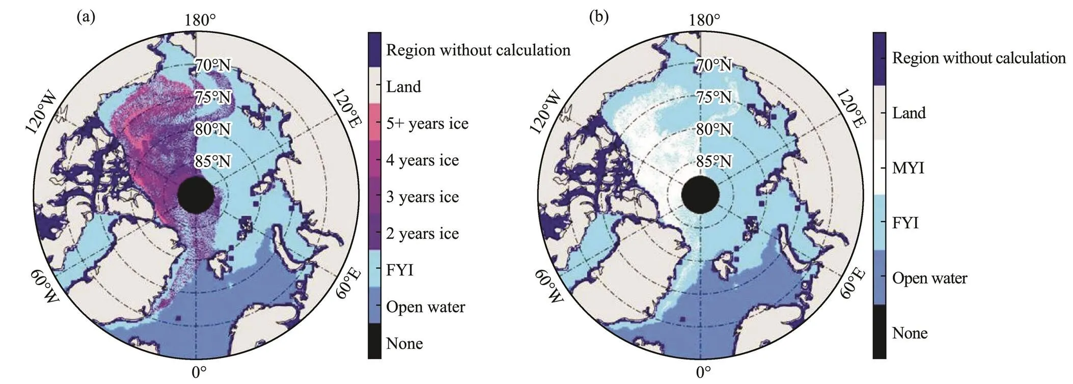
Fig.19 Sea ice type images in the 13th week of 2014. (a), EASE-Grid sea ice type; (b), NN sea ice type.

Fig.20 Time series of the MYI extent. The gray part indicates the period from June to September without NN classification.
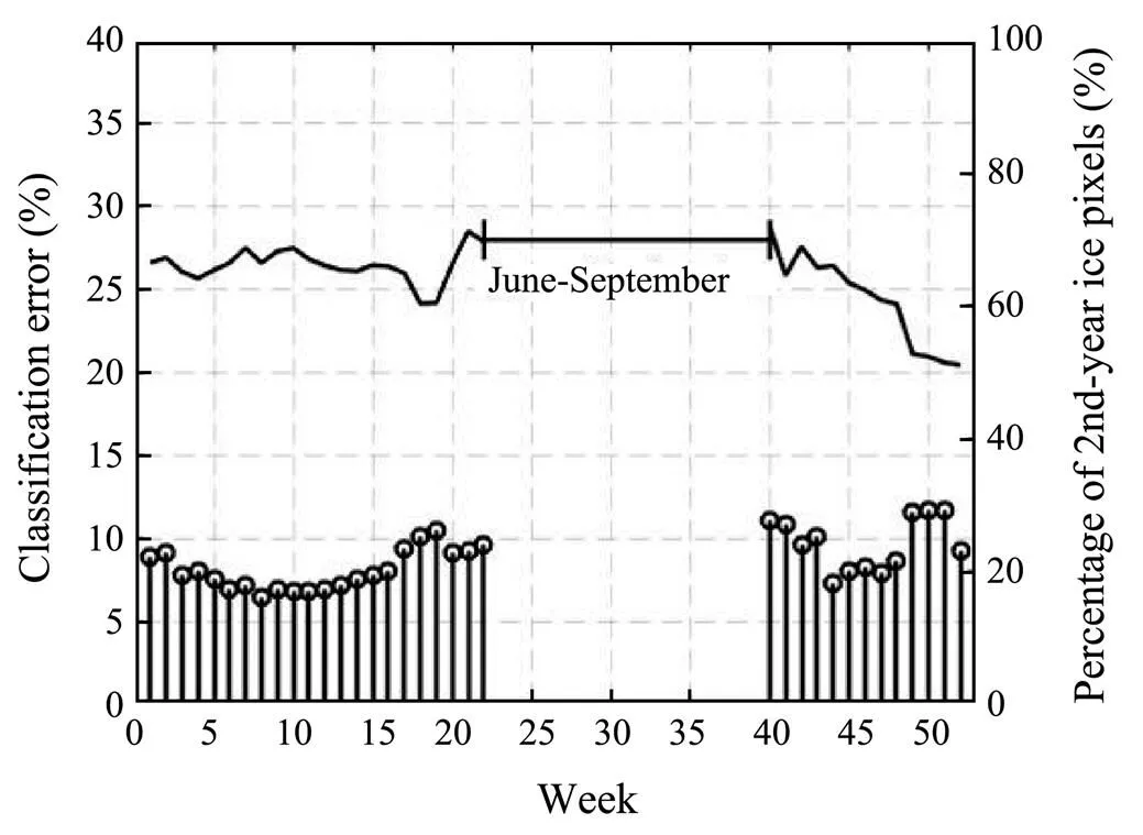
Fig.21 Sea ice classification error stem diagrams and percentages of second-year ice pixels. The stem plot represents the classification error, and the solid line represents the percentages of second-year ice pixels.
4 Conclusions
Based on the HY-2A/SCAT data, this paper employed a Bayesian sea ice detection algorithm to detect polar sea ice from January 1, 2014 to December 31, 2014, and applied a BP neural network to classify Arctic sea ice types from January to May and October to December in 2014.
For sea ice detection, the linear sea ice model parameter and ice backscatter variance (var[0 ice,]) that are suitable for the HY-2A/SCAT are obtained, in which the suitable tolerance factormixis 2 and the slope of the ice model is 1.09 with an offset of −0.49. HY-2A/SCAT daily sea ice extent maps in 2014 were then obtained based on these parameters.
For the validation of ice identification results, the AMSR2 sea ice concentration data were used to verify the detection results obtained by the Bayesian sea ice detection algorithm. The sea ice extent of the Bayesian sea ice detection algorithm was in good agreement with the AMSR2 ice extent defined by the 15% ice concentration isoline in the ice growth season, while the Bayesian sea ice detection algorithm detected a wider ice edge than the AMSR2 in the ice melting season. Previous studies have proved that the AMSR sea ice extent is reliable in the ice growth season but may be underestimated in the melting season (Markus and Cavalieri, 2000). Therefore, the performance of the Bayesian sea ice detection algorithm with the HY- 2A/SCAT is comparable to that of the AMSR2 during the ice growth season. As for the sea ice melting season, Rivas and Stoffelen (2011) used high-resolution visual satellite products to prove that the Bayesian sea ice detection algorithm was good at detecting diffuse ice during the melting period. The better detection ability enables the Baye- sian sea ice detection algorithm to estimate the sea ice edge more conservatively, which indicates that the relatively wider HY-2A/SCAT ice edge derived from the Bayesian sea ice detection algorithm compared with the AMSR2 result is reasonable.
For the sea ice type classification, HY-2A/SCAT data from January to May and October to December in 2013 were used for BP neural network modeling. A 5-9-1 neural network was applied to classify the Arctic sea ice type from January to May and October to December in 2014, in which the input parameters of the neural network include backscattering coefficients and one week number. HY-2A/SCAT sea ice type results were validated by EASE- Grid sea ice age products. The comparison showed that the variation of the FYI extent had the same tendency as the total sea ice extent, reflecting the seasonal melting and freezing characteristics of FYI. The trend of the MYI extent was consistent with that of the EASE-Grid. Compared with the EASE-Grid, the HY-2A/SCAT underestimated the MYI extent with an average classification error of 8.6%. Most misclassified pixels are unidentified second- year ice types, and the number of unidentified second-year pixels accounts for more than 50% of all misjudgement points for each week, indicating that the NN sea ice type classification is weaker in identifying younger multi-year ice.
In future work, the existing sea ice identification and sea ice type classification algorithms will be further inves- tigated, especially using visual satellite images or SAR images to further verify the sea ice detection capability in the sea ice melting season. Moreover, the authors plan to integrate different reliable sea ice type products such as Canadian Ice Service ice charts to use the scatterometer data in classifying sea ice types and sea ice identification in the future. In addition, other polar applications of scatterometers such as ice concentration and ice thickness (Egbers, 2019) also need further exploration.
Acknowledgements
The study is supported by the National Natural Science Foundation of China (No. 42030406). The authors would like to thank the Royal Netherlands Meteorological Institute (KNMI) for the Pencil Beam Wind Processor (PEN- WP) software, the National Satellite Ocean Application Ser- vice (NSOAS) for the HY-2A/SCAT Level 2A data, the National Snow and Ice Data Center (NSIDC) for AdvancedMicrowave Scanning Radiometer 2 (AMSR2) sea ice con- centration data and the Equal-Area Scalable Earth Grid (EASE-Grid) sea ice types data, and the European Centre for Medium-Range Weather Forecasts (ECMWF) for ERA 5 wind field data.
Bhowmick, S. A., Cotton, J., Fore, A., Kumar, R., Payan, C., Rodriguez, E.,, 2019. An assessment of the performance of ISRO’s SCATSAT-1 scatterometer., 117 (6): 959, DOI: 10.18520/cs/v117/i6/959-972.
Bi, H. B., Liang, Y., Wang, Y. H., Liang, X., Zhang, Z., Du, T.,., 2020. Arctic multiyear sea ice variability observed from satellites: A review., 38 (4): 962-984, DOI: 10.1007/s00343-020-0093-7.
Brath, M., Kern, S., and Stammer, D., 2013. Sea ice classification during freeze-up conditions with multifrequency scatte- rometer data., 51 (6): 3336-3353.
Brodzik, M. J., and Knowles, K., 2002. EASE-Grid: A versatile set of equal-area projections and grids. In:. Goodchild, M., and Kimerling, A. J., eds., National Cen- ter for Geographic Information and Analysis, Santa Barbara, USA, 98-113.
Chi, J., Kim, H. C., Lee, S., and Crawford, M. M., 2019. Deep learning based retrieval algorithm for Arctic sea ice concentration from AMSR2 passive microwave and MODIS optical data., 231: 111204, DOI: 10. 1016/j.rse.2019.05.023.
Egbers, H. N., 2019. Estimation of wintertime Arctic sea ice thick- ness with satellite scatterometers. Master thesis. Delft Univer- sity of Technology.
Goodfellow, I., Bengio, Y., and Courville, A., 2016.MIT Press, Cambridge, 800pp.
Haan, S. D., and Stoffelen, A., 2001. Ice discrimination using ERS scatterometer. OSI SAF Document KNMI-TEC-TN-120, EUMETSAT. Retrieved from: https://knmi-scatterometer-web- site-prd.s3-eu-west-1.amazonaws.com/publications/safosi_w_icescrknmi.pdf.
Heinrichs, J. F., Cavalieri, D. J., and Markus, T., 2006. Assessment of the AMSR-E sea ice-concentration product at the ice edge using RADARSAT-1 and MODIS imagery., 44 (11): 3070- 3080, DOI: 10.1109/TGRS.2006.880622.
Li, J., Cheng, J. H., Shi, J. Y., and Huang, F., 2012. Brief introduction of back propagation (BP) neural network algorithm and its improvement.,169: 553-558, DOI: 10.1007/978-3-642-30223-7_87.
Li, M. M., Zhao, C. F., Zhao, Y., Wang, Z. X., and Shi, L. J., 2016. Polar sea ice monitoring using HY-2A scatterometer measurements., 8 (8): 688-703, DOI: 10.3390/ rs8080688.
Lindell, D. B., and Long, D. G., 2016a. Multiyear Arctic ice classification using ASCAT and SSMIS.,8(4):294-313, DOI: 10.3390/rs8040294.
Lindell, D. B., and Long, D. G., 2016b. Multiyear Arctic sea ice classification using OSCAT andQUIKSCAT., 54(1): 167-175, DOI: 10.1109/TGRS.2015.2452215.
Long, D. G., 2017. Polar applications of spaceborne scatterometers., 10 (5): 2307-2320,DOI: 10. 1109/JSTARS.2016.2629418.
Markus, T., and Cavalieri, D. J., 2000. An enhancement of the NASA team sea ice algorithm., 38 (3): 1387-1398, DOI: 10.1109/ 36.843033.
Markus, T., and Cavalieri, D. J., 2009. The AMSR-E NT2 sea ice concentration algorithm: Its basis and implementation., 29 (1): 216-225.
Meier, W. N., Markus, T., and Comiso, J. C., 2018. AMSR-E/ AMSR2 unified L3 daily 12.5km brightness temperatures & sea ice concentration polar grids, version 1. NASA National Snow and Ice Data Center Distributed Active Archive Center. Boulder, USA, https://doi.org/10.5067/RA1MIJOYPK3P.
Nakata, K., Ohshima, K. I., and Nihashi, S., 2019. Estimation of thin-ice thickness and discrimination of ice type from AMSR- Epassive microwave data., 57 (1): 263-276, DOI: 10.1109/TGRS. 2018.2853590.
Nishio, F., and Comiso, J. C., 2005. The polar sea ice cover fromAqua/AMSR-E.. Seoul, 4933-4937.
Nishio, F., Comiso, J. C., Nakayama, M., and Gasiewski, A., 2004. Validation of AMSR-E ice concentration & thickness in the Okhotsk Sea., 68 (2): 439-443, DOI: 10.4067/S0717- 65382004000300022.
Otosaka, I., Rivas, M. B., and Stoffelen, A., 2018. Bayesian sea ice detection with the ERS scatterometer and sea ice backscatter model at C-band., 56 (4): 2248-2254.
Pearson, F., 1990.CRC Press, Boca Raton, 372pp.
Portabella, M., and Stoffelen, A., 2006. Scatterometer backscatter uncertainty due to wind variability., 44 (11): 3356-3362, DOI: 10.1109/TGRS.2006.877952.
Remund, Q. P., and Long, D. G., 1997. Automated Antarctic ice edge detection using NSCAT data.–. Singapore, 1841-1843.
Remund, Q. P., and Long, D. G., 1999. Sea ice extent mapping using Ku band scatterometer data., 104 (C5): 11515-11527.
Remund, Q. P., and Long, D. G., 2014. A decade of QUIKSCAT scatterometer sea ice extent data., 52 (7): 4281-4290, DOI: 10.1109/ TGRS.2013.2281056.
Ren, S. H., Liang, X., Sun, Q. Z., Yu, H., Tremblay, L. B., Mai, X. P.,., 2021. A fully coupled Arctic seaice-ocean-atmo- sphere model (ArcIOAM v1.0) based on C-Coupler2: Model description and preliminary results., 14 (2): 1101-1124, DOI: 10.5194/gmd-14-1101-2021.
Rivas, M. B., and Stoffelen, A., 2009. Near real-time sea ice dis- crimination using seawinds on QUIKSCAT. OSI SAF CDOP- KNMI-TEC-TN-168, EUMETSAT Ocean and Sea Ice SAF. Retrieved from: https://cdn.knmi.nl/system/data_center_pub- lications/files/000/068/084/original/sea_ice_osi_saf_final_re- port.pdf?1495621021.
Rivas, M. B., and Stoffelen, A., 2011. New Bayesian algorithm for sea ice detection with QUIKSCAT., 49 (6): 1894-1901, DOI: 10. 1109/TGRS.2010.2101608.
Rivas, M. B., Verspeek, J., and Verhoef, A., 2012. Bayesian sea ice detection with the advanced scatterometer ASCAT., 50 (7): 2649- 2657, DOI: 10.1109/TGRS.2011.2182356.
Sandven, S., Johannessen, O. M., and Kloster, K., 2006.. The American Society for Pho- togrammetry and Remote Sensing, Maryland, USA, 241-283.
Scott, K. A., Buehner, M., Caya, A., and Carrieres, T., 2013. A preliminary evaluation of the impact of assimilating AVHRR data on sea ice concentration analyses., 128: 212-223, DOI: 10.1016/j.rse.2012.10.003.
Snyder, J. P., 1987.–. U.S. Government Printing Office, Washington, D. C., 383pp.
Spencer, M. W., Wu, C., and Long, D. G., 2000. Improved resolution backscatter measurements with the SeaWinds pencil- beam scatterometer., 38 (1): 89-104, DOI: 10.1109/36.823904.
Swan, A. M., and Long, D. G., 2012. Multiyear Arctic sea ice classification using QUIKSCAT., 50 (9): 3317-3326, DOI: 10.110 9/TGRS.2012.2184123.
Tonboe, R., and Toudal, L., 2005. Classification of new-ice in the Greenland Sea using satellite SSM/I radiometer and Sea- Winds scatterometer data and comparison with ice model., 97 (3): 277-287.
Tschudi, M., Meier, W. N., Stewart, J. S., Fowler, C., and Mas- lanik, J., 2019. EASE-Grid sea ice age, version 4. January 1, 2013 to December 31, 2014. NASA National Snow and Ice Data Center Distributed Active Archive Center. Boulder, USA. DOI: 10.5067/UTAV7490FEPB.
Tucker, W. B., Perovich, D. K., Gow, A. J., Weeks, W. F., and Drinkwater, M. R., 1992. Physical properties of sea ice relevant to remote sensing. In:. Carsey, F. D., ed., American Geophysical Union, 9-28.
Vogelzang, J., Stoffelen, A., Verhoef, A., and Figa-Saldaña, J., 2011. On the quality of high-resolution scatterometer winds., 116 (C10): C10033, DOI: 10.1029/2010JC006640.
Wang, X. N., Liu, L. X., Shi, H. Q., Dong, X. L., and Zhu, D., 2012. In-orbit calibration and performance evaluation of HY- 2 scatterometer.. Munich, 4614-4616, DOI: 10.1109/ IGARSS.2012.6350438.
Wang, Z. X., Stoffelen, A., Fois, F., Verhoef, A., Zhao, C. F., Lin, M. S.,, 2017a. SST dependence of Ku- and C-band back-scatter measurements.,10 (5): 2135- 2146, DOI: 10.1109/JSTARS.2016.2600749.
Wang, Z. X., Stoffelen, A., Zhao, C. F., Vogelzang, J., Verhoef, A., Verspeek, J.,., 2017b. An SST-dependent Ku-band geo- physical model function for RapidScat., 122 (4): 3461-3480, DOI: 10.1002/20 16JC012619.
Wentz, F. J., and Smith, D. K., 1999. A model function for the ocean-normalized radar cross section at 14GHz derived from NSCAT observations.,104 (C5): 11499-11514, DOI: 10.1029/98jc02148.
Worby, A. P., and Comiso, J. C., 2004. Studies of the Antarctic sea ice edge and ice extent from satellite and ship observations.,92 (1): 98-111, DOI: 10. 1016/j.rse.2004.05.007.
Zhang, Z. L., Yu, Y. N., Li, X. Q., Hui, F. M., Cheng, X., and Chen, Z., 2019. Arctic sea ice classification using microwave scatterometer and radiometer data during 2002–2017., 57 (8): 5319- 5328, DOI: 10.1109/TGRS.2019.2898872.
Zhao, K., and Zhao, C. F., 2019. Evaluation of HY-2A scatterometer ocean surface wind data during 2012–2018., 11 (24): 2968-2990, DOI: 10.3390/rs11242968.
Zou, J. H., Zeng, T., Guo, M. H., and Cui, S. X., 2016. The study on an Antarctic sea ice identification algorithm of the HY-2A microwave scatterometer data., 35 (9): 74-79, DOI: 10.1007/s13131-016-0927-5.
January 4, 2021;
May 12, 2021;
June 10, 2021
© Ocean University of China, Science Press and Springer-Verlag GmbH Germany 2022
. E-mail: zhaocf@ouc.edu.cn
(Edited by Chen Wenwen)
 Journal of Ocean University of China2022年2期
- Journal of Ocean University of China的其它文章
- Study of the Wind Conditions in the South China Sea and Its Adjacent Sea Area
- A Spatiotemporal Interactive Processing Bias Correction Method for Operational Ocean Wave Forecasts
- Characteristics Analysis and Risk Assessment of Extreme Water Levels Based on 60-Year Observation Data in Xiamen, China
- Underwater Target Detection Based on Reinforcement Learning and Ant Colony Optimization
- Thermo-Rheological Structure and Passive Continental Margin Rifting in the Qiongdongnan Basin,South China Sea, China
- Effect of Penetration Rates on the Piezocone Penetration Test in the Yellow River Delta Silt