
Shedding vortex simulation method based on viscous compensation technology research
2022-04-12 03:44HaoZhou周昊LeiWang汪雷ZhangFengHuang黄章峰andJingZhiRen任晶志
Chinese Physics B 2022年4期
Hao Zhou(周昊) Lei Wang(汪雷) Zhang-Feng Huang(黄章峰) and Jing-Zhi Ren(任晶志)
1Department of Mechanics,Tianjin University,Tianjin 300072,China
2Science and Technology on Space Physics Laboratory,China Academy of Launch Vehicle Technology,Beijing 100076,China
Keywords: shedding vortex,viscosity analysis,numerical dissipation,turbulence models
1. Introduction
The turbulence phenomenon is widely used in a large number of engineering studies ranging from aeronautical aircraft to biomedical equipment. Understanding and accurately predicting the formation and evolution mechanism of vortex structure plays an important role in solving modern engineering design problems.[1]Owing to the particularity of the helicopter rotor structure, the shedding vortex generated by a single blade contacting the adjacent blade will cause new mechanical problems.[2]To capture shedding vortexes accurately and obtain related microscopic information,it is necessary to divide millimeter-scale fine mesh in the vortex evolution region. Comparing with the vortex structure, the blade size is much larger, and the boundary length of the calculated domain usually reaches several meters or even tens of meters.[3]Because in the actual engineering research,there is need to consider the requirements for calculation time and calculation efficiency. If the outflow field grid is encrypted, it takes a too long time to be calculated by traditional simulation methods,which is obviously unacceptable in engineering applications.[4]Therefore,the dense grid is arranged only near the boundary layer on the airfoil wall and in a vortex generation region. In the vortex evolution region at the far end of the flow field, the grid size gradually increases. In this case, the grid form can measure only the variation of parameters such as lift resistance,pressure,and St on the wall.[5-7]The sparse mesh is no longer matched with the actual size of the vortex,resulting in the dissipation or even disappearance of the vortex.The two-dimensional rotor aerodynamics of propeller vortex interaction cannot be further studied.
The current research focuses on developing a variety of grid forms to improve the accuracy of small-scale flow structure simulation. For example, Yanget al.[8]proposed an overlapping grid technology and multi-grid algorithm. This method was applied to the numerical simulation of the viscous flow around a hovering rotor, indicating that the calculation time is reduced. Xuet al.[9]combined the overlapping mesh technique with the weighted essentially nonoscillatory scheme to improve the ability to capture vortices.Xia and Yang[10]developed an unsteady numerical simulation method based on dynamic surface grid construction technology to solve the problems related to propeller vortex interference. Tanget al.[11]developed a new MFBI algorithm to solve the problem about low efficiency in the location calculation of three-dimensional complex structures overlapping grids. Markuset al.[12]used vortex-adapted Chimera child grids to achieve a local refinement of the grid in the vicinity of the vortex, and thus reducing the numerical dissipation of the vortex. Nathan[13]used the fifth-order/seventh-order spatially accurate ENO scheme in conjunction with overset vortex refinement to improve the accuracy of wing-tip vortex measurements for blunt wing tips. Unfortunately, the above methods were applied only to certain models and incoming flow conditions. And the grid distribution needs to be adjusted in real time according to the evolution process of the vortex. This method has poor universality and high operation difficulty, so it is not suitable to being popularized in the engineering field. Therefore, it is urgent to develop an efficient vortex shedding simulation method for practical engineering research. Based on changing no grid form,the corresponding engineering requirements can be achieved by optimizing the calculation method.
Up to now, Reynolds-averaged Navier-Stokes (RANS)equation is still the most commonly used numerical simulation method in aerodynamic design. However, for many complex flow phenomena, satisfactory results cannot be obtained by the traditional RANS method. With the continuous development of turbulence model theory,researchers have found that the viscosity coefficient contained in the RANS model is not necessarily universal, and the optimal value usually depends on the actual problem.[14]For example, the low-Reynoldsnumberk-εtwo-equation turbulence model can simulate more complex flows than the zero-equation. However, it cannot correctly predict the influence of a solid wall boundary on turbulence.[15]Wilcox[16]proposed thek-ωmodel to overcome the shortcomings of thek-εmodel, enabling accurate simulations of the flow state near the wall surface. The turbulent viscosity is expressed as
The Wilcoxk-ωmodel also has certain limitations. Its simulation accuracy for low Reynolds numbers, compressibility,and shear flow propagation needs to be improved.[17]These problems have been solved by using a correction coefficientα∗and other developments of the standardk-ωmodel. In this case,the expression for the turbulent viscosity is modified into
Menter[18]then developed the shear-stress transport(SST)kωturbulence model,which combines thek-ωandk-εmodels by using a switching function.By further modifying the turbulent viscosity,the new model achieves a good simulation effect in different regions near the wall and at the far end of the flow field. In the SSTk-ωformulation, the turbulent viscosity is expressed as

To sum up, the development of turbulence model theory provides us with good inspiration. Since the vortex is greatly affected by the viscosity of the flow field in the evolution stage, the influence of grid-scale on the flow field can be analyzed and quantified. The theoretical relationship between mesh scale and flow field viscosity is established to correct the relative parameters in the traditional turbulence model. The above-mentioned idea is referred to as viscosity compensation correction method. This method solves the problem that the traditional grid method cannot accurately simulate the evolution process of shedding vortex. At the same time, the efficiency of vortex simulation is improved,and it can be applied to engineering practice as well.
The remainder of this paper is organized as follows. The theoretical framework of the viscous compensation correction method is established in Section 2. Detailed normative verification based on the flow around a single-cylinder model is presented in Section 3. To verify the universality of the method and further modify the NACA0012 (National Advisory Committee for Aeronautics 0012) airfoil and doublecylinder model in Section 4. Finally, the correction effects of three typical flows around the problem are summarized and the conclusions are drawn in Section 5.
2. Turbulent viscosity adaptive correction model
2.1. Theoretical analysis
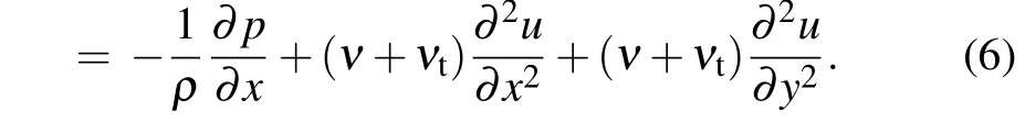
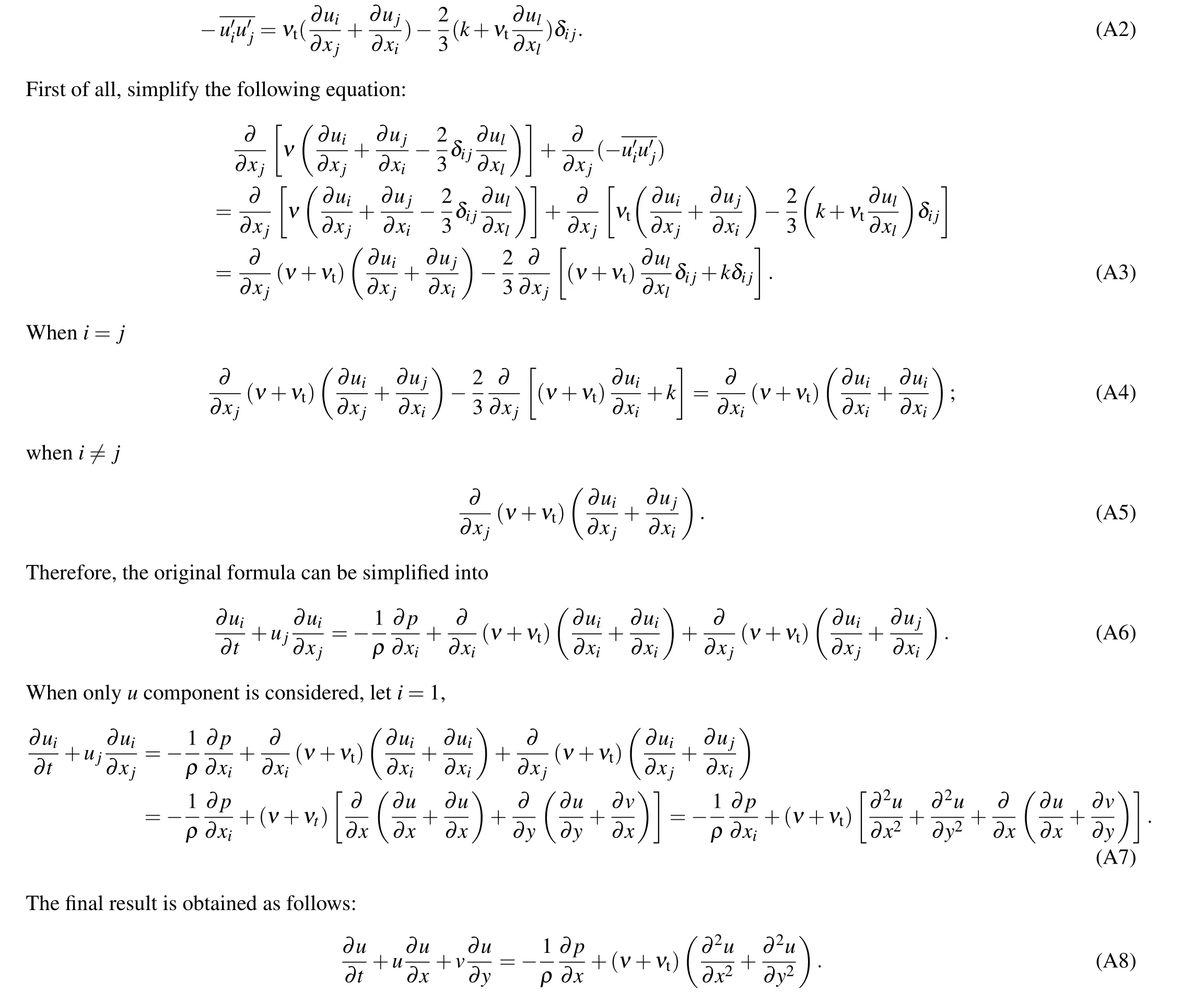
In engineering,Reynolds averaging is used to simplify the two-dimensional steady-state incompressible Navier-Stokes equations and obtain the RANS equations. Withνdenoting the physical viscosity of the fluid, which is an inherent characteristic,[19]we can write

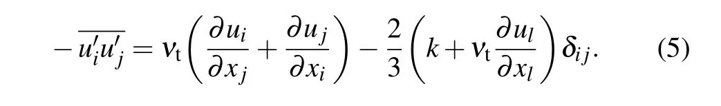
In this equation, additional conditions caused by turbulence are exposed and must be simulated to close the equation. Using the Boussinesq hypothesis,the second-order correlation of velocity pulsation is expressed as the product of average velocity gradient and turbulent viscosity coefficient. Turbulent viscosity coefficientνtis related to a reaction of fluid flow rather than a physical property of the fluid,[20]satisfying the following equation:
After simultaneous simplification, the differential equation containing the physical viscosity coefficient and the turbulent viscosity coefficient can be obtained. Only the velocity componentuis taken for example,and componentvhas a similar form to componentu,so it will not be described in detail here. The detailed derivation of the following equation can be found in Appendix A:
In addition to physical viscosity and turbulent viscosity,numerical viscosity is also introduced into the process of solving differential equations. In most of cases, it is very difficult to solve the partial differential equations directly. It is necessary to arrange corresponding grids in the calculation area to discretize the continuous field of physical quantity.[21]Therefore,continuous partial differential equations can be discretized into algebraic equations on a computational grid according to some difference scheme. Then the numerical solution is obtained by simulation. Its accuracy depends on the difference scheme used, and its error is closely related to the grid-scale.[22]For example, the velocity componentuin the differential equation is discretized by using the first-order upwind scheme:
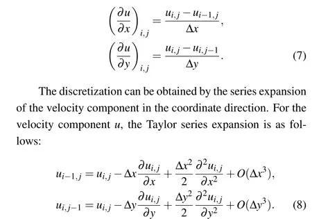
Any expansion can include only a certain number of terms.Therefore,a discretized truncation error is generated,and this is often called numerical viscosity.[23]By substituting the discretized equation into the original differential equation, the first-order upwind scheme difference equation can be obtained as follows:
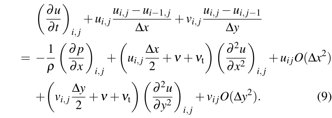
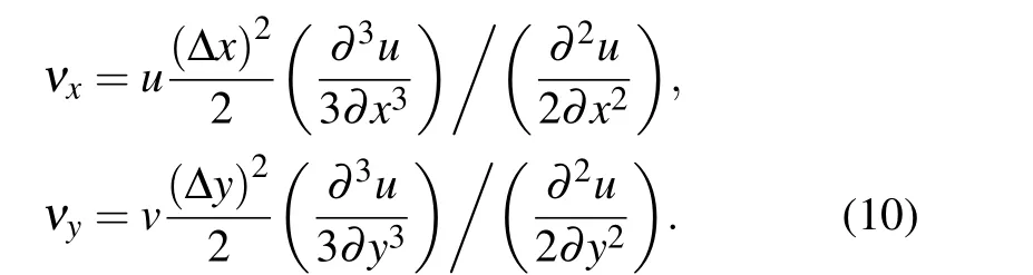
At this point,the differential equation of Eq.(6)is transformed into the difference equation of Eq. (9) by the discretization scheme. Letνxandνyrepresent the numerical viscosity coefficients of the two coordinate directions,respectively. Then, the numerical viscosity of the first-order upwind scheme can be expressed asνx=uΔx/2,νy=vΔy/2.Similarly, the velocity componentucan be discretized in a second-order upwind format and expanded into a Taylor series. The numerical viscosity expression of the second-order upwind scheme can then be obtained to be
The grid is the basis of discretization and plays a key role in implementing the discretization. When simulating the evolution process of shedding vortices, the accuracy can be improved by reducing the mesh spacing, although this will increase the computational burden. Conversely, reducing the number of grid cells can reduce the computational cost. However, the numerical dissipation will increase and the strength of the shedding vortices will weaken.[24]Since the numerical viscosity is closely related to the local velocity and the local grid-scale, the numerical dissipation caused by the increase of grid-scale is called the grid viscosity dissipation. Its effect is approximately analogous to numerical viscosity, resulting in the increase of the total viscosity of the flow field.When an aircraft moves at high speed, its physical viscosity is very small. Therefore, the viscosity compensation correction method does not involve physical viscosity. However, at this time, the turbulence phenomenon is obvious, and turbulence viscosity plays a significant role.[25]At the same time,the numerical viscosity can be combined with the physical viscosityνand the turbulent viscosityνt. These three kinds of viscosities together drive and affect the evolution of the shedding vortices. Therefore, mesh viscosity can be regarded as hidden in turbulent viscosity. As the mesh size increases, the total viscosity in the flow field increases, and the dissipation of shedding vortexes is intensified. Let Δrrepresent the local grid scale,then the turbulence viscosity coefficient will be modified by constructing the mesh scale function to reduce the numerical dissipation:
2.2. Method establishment
The core of the viscosity compensation correction method is to establish the relationship between mesh size and numerical viscosity. Using this relationship, the specific expression of the correction functionf(Δr)can then be determined. The Reynolds number is used to characterize the motion of a fluid.It is proportional to the characteristic velocity and the characteristic length. Therefore,a new variable is created in the form of the Reynolds number-the grid Reynolds number(ReC)as shown below:

The effect of grid-scale on flow field is changed from abstract to concrete.
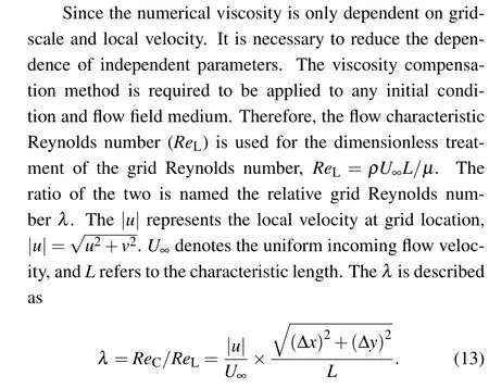
For engineering problems, unstructured hybrid grids are generally used to simulate the flow field characteristics of complex structures. To better meet the engineering requirements, this method also modifies the flow field of unstructured grids. The grid shape is irregular,and the grid-scale along theXandYcoordinate axes cannot be accurately measured. Therefore, the direction of the grid-scale is not discussed for calculation purposes, but isotropy is considered. The two-dimensional gridscale is approximately the square root of the local grid area.Letν1andν2represent the numerical viscosity coefficient of the simplified first-order scheme and second-order scheme,respectively,then they will be expressed as
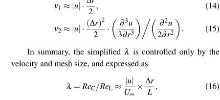
and thus has similar properties to the numerical viscosity.
The mesh viscosity correction coefficientαcellis constructed by combiningλand two undetermined coefficientsC1andC2, which are used to measure the influence of mesh scale on the flow field. The two parameters are placed at the exponential position and factor position ofλrespectively,corresponding to the numerical viscosity coefficients of each difference scheme. This ensures that the mesh viscosity and numerical viscosity have similar forms.
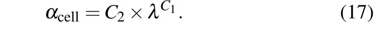
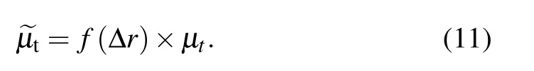
Finally,αcellis used to construct the correction function to adjust the turbulent viscosity coefficient. The mesh viscosity,which is considered to be hidden in the turbulent viscosity,is removed to reduce the total viscosity of the flow field and make up for the lack of unsteady information. The core equation of the viscosity compensation correction method is as follows:

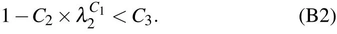
There are three undetermined parameters in Eq.(18),and the basis for their values should be clarified. First,λis affected only by the velocity and grid size. Therefore,C1should be consistent with the index values of the two physical quantities. In the expression ofν1, the velocity has a linear relationship with the grid-scale, soC1=1. In the expression ofν2, the grid-scale is squared and the velocity term is the ratio of the third derivative to the second derivative. Therefore,C1should take a value between 1 and 2.C2helps adjust the correction quantity of different density meshes. In principle,the turbulence model modification should be controlled in a reasonable range. In this way, the properties of the flow field are not changed by the introduction of the method. The value ofαcellrises as the mesh size increases,resulting in a continuous decrease in the correction factor, which may potentially become negative. Therefore, the correction is limited by the introduction of a further parameterC3(see Appendix B).
3. Validation of single-cylinder model
3.1. Calculation model
The diameter D of the single-cylinder model is 1 m(see Fig. 1). The center of the circle is placed at the origin of the coordinate axes. The cylindrical surface has no-slip and no-penetration boundary conditions. The calculation area is 25D×10D. The upstream velocity inlet and the downstream pressure outlet are 5Dand 20Daway from the center of the circle,respectively.Both the upper boundary and lower boundary are both 5Daway from the center of the circle. These calculation domain settings have little influence on the flow field results.[26]
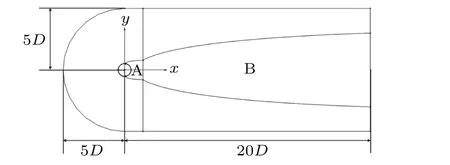
Fig.1. Single cylinder model grid partition.
Hybrid grids can improve the quality of the computational mesh and reduce the difficulty in discretizing the regional mesh. Complex computing domains can be efficiently discretized, saving time and computer resources.[27]Therefore,A region and B region are divided into mixed meshes with different densities. First of all,vortices are generated and shed near the model wall.The processing method of this region will significantly affect the results of numerical simulation.[28]The high-density structured grid is arranged near the wall boundary layer, while the small-scale unstructured dense grid is arranged in region A.The first layer of the mesh in the boundary layer is perpendicular to the wall surface,and the mesh height is about 0.25 mm(see Fig.2).

Fig.2. Near-wall grid model.
Region B of the same flow around the model is divided into several sets of grids with increasing meshes. The maximum mesh size of each grid in the B region is about one order of magnitude larger than the minimum mesh size. As a result, the shedding vortex has a different degree of dissipation. It is worth noting that after verifying the grid independence for both the wall boundary layer region and the A region, the grid of the two regions is kept unchanged.[29]In this way, the difference in vortex shape is caused only by the different grid scales in region B.The large-scale unstructured grids are used in the rest of the irrelevant regions,and the grids at the junction of the regions are smooth. A reference point is set atX=18Dto monitor the changes in vorticity peak values with each grid, allowing the correction effect of the viscous compensation method to be verified.
In the modeling process,the left boundary inlet surface is set as the velocity inlet, and the fluid medium is air. We setU=50 m/s,V=0 m/s, the turbulence intensityI=2.45%,and the turbulence viscosity ratio to be 10. The right boundary outflow surface is set as the pressure outlet,and the upper and lower boundary conditions are symmetric. For incompressible flows,a pressure-coupled solver needs to be selected. The PISO algorithm and the second-order upwind format[30]are used in consideration of the computational accuracy and calculation time. The SSTk-ωturbulence model is used to simulate the flow around the cylinder. The convergence criterion of the continuity equation residuals is set to be 10-5. The time interval for unsteady computations is 0.0005 s, and each step is iterated up to 30 times.
3.2. Grid-scale coefficient
According to Eq.(16),λis controlled by the speed ratio and the mesh scale ratio. The change in these two parameters is monitored at different positions on thexaxis.The results are shown in Fig. 3. The grid is relatively dense in the near-wall region and region A, with Δr ≪L. Here, the velocity at the wall position is 0, and the normal velocity gradient is large.Thus,λis affected by both the velocity ratio and the length ratio. At the same time, the numerical dissipation caused by high mesh density is small,so the influence degree of the viscous compensation method in the near field region is limited.On the contrary,in region B,which is the focus of this paper,the increase of mesh size leads the mesh viscosity to increase.The shedding vortex dissipation is obvious,which is the core area of the viscosity compensation method. At this point,the local velocity tends to be stable and the ratio concerning the incoming flow velocity is close to 1. However, there is still a significant gap between the local grid-scale and the characteristic length. Thus,in this region,λis dominated by the length ratio.
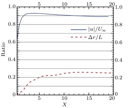
Fig.3. Parameter ratios at different positions.
To describe the density of the mesh more conveniently,λis simplified into the ratio of the gridscale to the characteristic length at different positions in region B.The gridscale coefficient is established and expressed byβ,
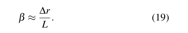
The grid scale of the dense mesh and the coarse mesh are respectively expressed asβ1andβ2, which satisfy the relationβ1<β2.
3.3. Numerical simulations
First of all,it is necessary to obtain the exact solution of the peak vorticity as a standard value for subsequent verification and comparison. The method is to gradually encrypt the grid in region B until the peak vorticity no longer changes with the decrease of grid size(see Fig.4). When the total number of meshes is 1.6×10⁵,the exact solution of the vorticity peak is obtained, which is about 20 s-1. The grid is named grid 1 with grid-scaleβ ≈0.025.
Subsequently,the number of grid cells in region B is gradually reduced,so that the maximum grid-scale differs from the minimum one by about one order of magnitude. Three sets of grids,i.e., grid 2, grid 3, and grid 4, are used to verify the correction effect. The total number of grid cells is 5×104,4.2×104, and 4×10⁴for gird 2, grid 3, and grid 4, respectively. The corresponding grid-scale coefficients areβ=0.2,0.25,and 0.35(see Fig.5).
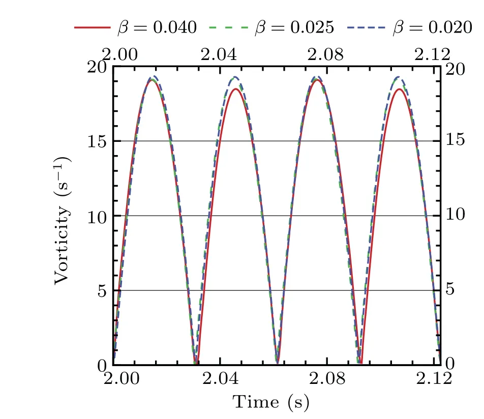
Fig.4. Vorticity peak comparison in a dense mesh.
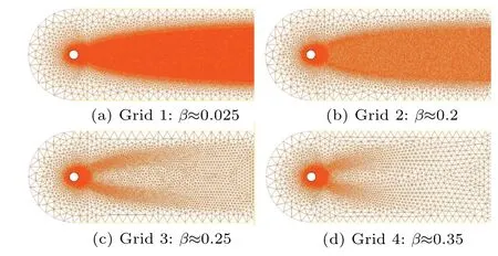
Fig.5. Single cylindrical grid.
3.4. TVAC model effect verification
Referring to the parameter value method in Appendix B,the final calculation results areC1=1.8,C2=35, andC3=0.1. The viscous compensation method is used to simulate each grid, focusing on the comparison of the area and intensity peak of the far-end vortex. First of all,qualitative analysis is made according to the change of the vorticity cloud chart.The two columns represent the results before and after compensation respectively(see Fig.6). By comparison,it is found that some shedding vortices can be seen in the front of region B with the decrease of the number of grids before correction.In the process of backward propagation,the area of the vortex becomes smaller and the color becomes lighter. Near the exit of the flow field,the dissipation of the shedding vortex is obvious or even disappears. After correction,the areas of the three grid vortices increase. On a maximum grid-scale, the shedding vortices which originally dissipate and disappeare and appear again, qualitatively showing that the correction effect has reached an expected value.

Fig.6.Single-cylinder model vorticity contours before and after corrections.

Fig.7. Peak vorticity before correction.
The variation of vorticity peak at the reference point is analyzed quantitatively. Before the correction,the peak value of vorticity decreases with the increase of grid-scale. The modified grid 2 vorticity peak is very close to the exact solution of the dense grid. At the same time,the peak value of grid 3 vorticity is also significantly improved. Owing to the large scale of grid 4, the far-field shedding vortex has completely disappeared. The viscous compensation method cannot be completely compensated for, which leads to a certain difference between the corrected peak value and the accuracy. However,the relative error is significantly reduced from 45.2%to 29.6%.The peak value of vorticity increases obviously,which reflects the effectiveness of the method to a certain extent(see Figs.7 and 8).
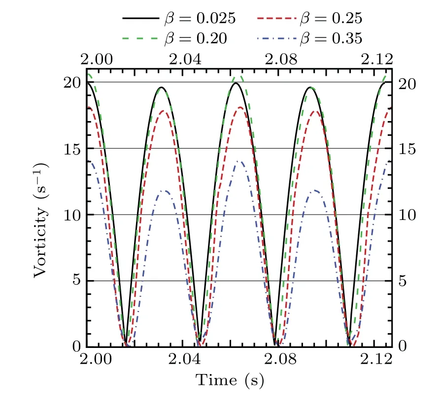
Fig.8. Peak vorticity after correction.
Finally, if the shedding vortex propagates backward for one second, only one-third of the time required for the dense grid is taken after coarse grid correction(Table 1). The results show that when the difference in grid size is about ten times,the viscous compensation method can ensure the calculation accuracy and improve the calculation efficiency significantly.
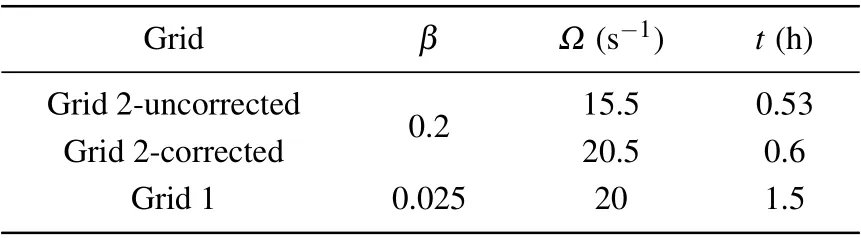
Table 1. Single cylinder model correction effect.
4. Validation of other models
4.1. NACA0012 airfoil
The viscous compensation method is used to solve the NACA 0012 airfoil problem, with the original calculation conditions kept unchanged. When the distance between the boundary of the computational domain and the wall is more than 3 times the chord length,it has little effect on the simulation results.[31]Consider the airfoil chord as the characteristic lengthL,then the left boundary and the right boundary are 10Land 20Lfrom the center of the circle,respectively,and both the upper boundary and lower boundary are 10Lfrom the center of the circle(see Fig.9). According to the literature,when the angle of attack is greater than 13°,a separate vortex structure will appear on the leeward side of the airfoil.[32]When the angle of attack is 20°, the phenomenon of vortex shedding and backward propagation are both obvious. Therefore,the angle of attack is set to be 20°.
Following the grid distribution of the single-cylinder model, the grid of region B is gradually refined. The peak vorticity of the reference point converges on grid 1. The exact solution is 17.86 andβ ≈0.025. Increasing the grid-scale leads grids 2 and 3 to contain 5.3×10⁴and 5×10⁴cells,respectively,and haveβ ≈0.30 and 0.40(see Fig.10).
The viscous compensation method is used to test each grid. First,the changes in the vorticity cloud images are compared(see Fig.11). After correction,the intensity and the area of the shedding vortices increase. In grid 3,the shedding vortices near the exit are reproduced. This shows that this method can solve the problem about the flow around NACA0012 airfoil.
The changes in peak vorticity at the reference point are monitored. Before the correction,the peak values of vorticity for grids 2 and 3 are obviously lower,22.2%and 30.6%lower than the exact solution, respectively. After correction, their peak vorticity values increase and their grid-scale differences are more than one order of magnitude larger than before correction By increasing the compensation, the maximum grid has a better correction effect. Although the grid 2 vorticity peak will slightly exceed the exact solution,the error of grid 3 can be significantly reduced to 4.6%.
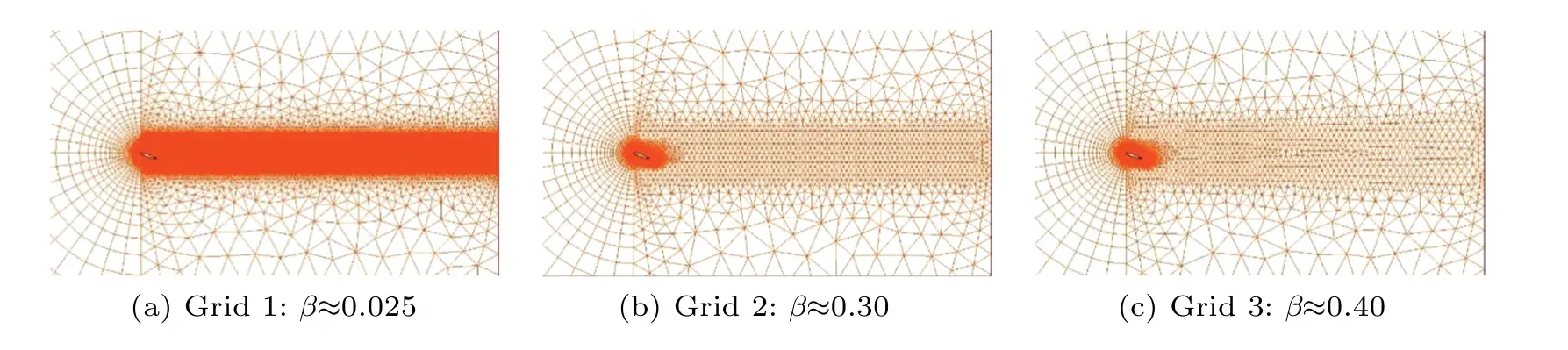
Fig.10. NACA0012 airfoil grids.

Fig.11. NACA0012 model vorticity contours before and after corrections.
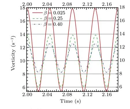
Fig.12. Peak vorticity before correction.
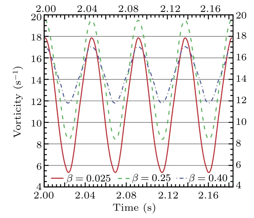
Fig.13. Peak vorticity after correction.
According to the statistics in Table 2, it takes only onethird of the time for the coarse grid to reach the same accuracy, which significantly improves the computational efficiency. Therefore,the viscous compensation method is effective in correcting the flow around NACA 0012 airfoil.
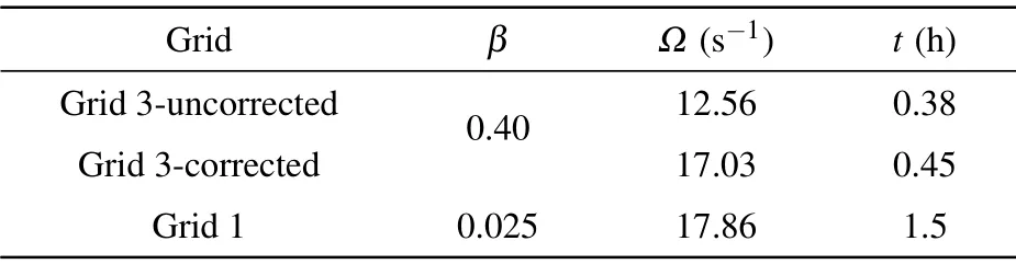
Table 2. NACA0012 airfoil compensation effect.
4.2. Double-cylinder model
The center of the front cylinder is placed at the origin of the coordinate axis. The center of the rear cylinder is located on theXaxis,10Daway from the front cylinder(see Fig.14).Like a single cylinder,a dense grid is arranged in region A near the wall. It is worth noting that the model focuses on the flow region B between two cylinders,and several grids are assumed to have different densities. Unstructured grids are arranged in the flow field region C and other irrelevant areas outside the rear cylinder,and the grid size increases gradually.
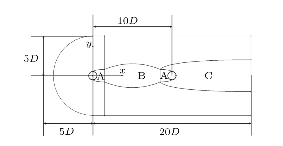
Fig.14. Double cylinder model grid partition.
The simulation results of meshes with different densities have different effects on the strength of the shedding vortex,resulting in different stresses on the rear cylinder. Therefore,we need to investigate the changes of lift coefficient of the two cylinders before and after corrections. The lift coefficient(cl)is given as follows:
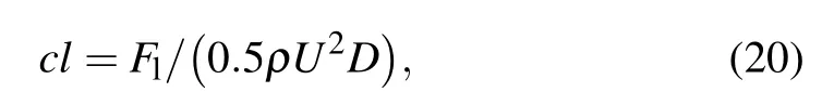
whereFlis the lift.

Fig.15. Double-cylinder grid.
The precise solution can be obtained by refining the region B grid: the lift coefficient on the front cylinder is about 1.306 and that on the back cylinder is about 1.959. At this time,the total number of grid cells is 1.2×10⁵(grid 1),with the maximum grid-scale is about 0.025. Then,grid 2 and grid 3 are obtained by increasing the grid spacing in region B.Their total numbers of grid cells are 2×10⁵and 1×10⁵, and their maximum grid-scale values are about 0.06 and 0.1, respectively(see Fig.15).
By comparing the vorticity cloud images (Fig. 16), it is clear that when the mesh is dense,the shedding vortices generated by the front cylinder are stronger and have better connectivity. As the grid size in region B increases, the size and intensity of the shedding vortices decrease, and the color in the figure becomes lighter. After correction, the intensity of the shedding vortices with the coarse mesh is improved. The color of the vortices in the figure is similar to that with the dense grid.

Fig.16. Double-cylinder model vorticity contours before and after corrections.
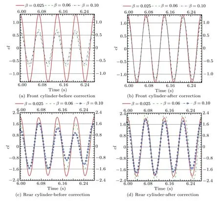
Fig.17. Lift coefficient amplitude correction effect before and after corrections.
The changes in the lift forces on the two cylinders are now analyzed in detail. As shown in Fig.17,before correction,the amplitude of cl on the two cylinders decreases as the grid size increases. Because the grid size of grid 3 is too large, the cl amplitude curve of the rear cylinder exhibits obvious fluctuations. After correction,the front cylinder compensation effect is very good. Moreover,the unstability of cl curve for the rear cylinder in grid 3 is improved. Stable amplitude results can be obtained,and these are approximately the same as the standard values.
Furthermore,a fast Fourier transform is applied to the rear cylinderclof grid 3. The results show that the viscous compensation method can effectively reduce the amplitude of the secondary frequency fluctuation and increase the amplitude of the primary frequency fluctuation(see Fig.18).The correction effect is again verified by analyzing this spectrum.
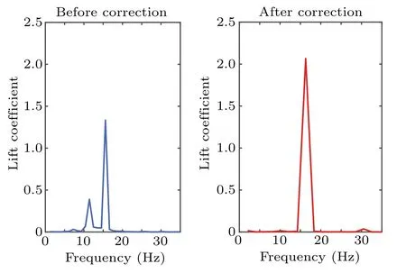
Fig.18. Amplitude-frequency curve correction effect.
By the viscous compensation method,for the rough mesh it takes only about 30%of the computation time of the dense mesh to achieve the same computational accuracy (see Table 3). All in all,this method effectively improves the lift coefficient amplitudes of the two cylinders and reduces the error between the model and the standard value, showing that the proposed method is effective in correcting the double-cylinder model.
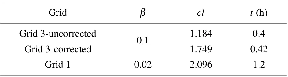
Table 3. Double cylinder model correction effect.
5. Conclusions
In practical engineering, a simulation method that can not only accurately simulate the evolution process of shedding vortex, but also save calculation cost is still being explored. This poses a great challenge to the traditional turbulence model framework, and there remain many unsolved problems. First, if only the grid type is considered, sliding grids are usually used to capture small-scale shedding vortices. The single grid form is effective only for specific models and conditions with poor robustness. Moreover, the grid construction process is more difficult and cannot be widely promoted in engineering applications. Second, the dissipation of the shedding vortex depends on the viscosity of the flow field. However, owing to the lack of relevant theoretical analysis, it is impossible to further study the internal mechanism and fundamentally solve the problem of vortex dissipation. Third,the grid scale is too large to capture the shedding vortex accurately,which is too abstract in concept. As theoretical research, we need to quantify the influence of grid-scale and build a credible theoretical framework.
At present,a large number of studies have confirmed that the turbulence model parameters can be modified appropriately according to the actual engineering requirements. In this work, we abandon the traditional method of modifying grid form and proceed directly from the formation mechanism of vortex dissipation. By comparing the grid dissipation with numerical viscosity quantitatively,the viscosity compensation method is established. Theλis the most important parameter to establish the relationship between grid viscosity and flow viscosity. Through the analysis, it is found that theλis controlled only by the grid-scale in the modified core region at the far end of the flow field. Therefore, in the process of modeling,theλcan be further simplified into grid-scale coefficientβ.
The viscous compensation method is verified through three different flow problems. The results show that when the maximum grid size of the correction area is about ten times in difference,the original vortex structure is regenerated at the far end of the flow field. At the same time, the peak value of vorticity and the amplitude of lift coefficient increase significantly, which reduces the error with respect to the standard value. Therefore,the computation time can be greatly reduced and the computation efficiency is improved. Finally,with the help of the viscous compensation method,the large-scale grid can be used to simulate the shedding vortex structure accurately and efficiently. Furthermore, the unsteady information can be obtained, which provides a new way for the followup study of helicopter rotor aerodynamics and aeroacoustics.With the the application range expanded and the algorithm optimized, the viscous compensation method will have a wider development prospect.
Appendix A:Derivation of differential equations
Given

Appendix B:Parameter determination method
The core correction equation of the TVAC model contains three undetermined parameters, and their values need to be clarified. Consider a certain model divided into three sets of grids, grids 1-3, with corresponding relative mesh Reynolds numbers ofλ1,λ2,andλ3,whereλ1<λ2<λ3.
First,C1is at the exponential position ofλ, and bothλand the numerical viscosity are affected only by the velocity and the grid scale. Therefore,C1should be consistent with the exponential position of the two parameters. For the firstorder scheme, there is a linear relationship between velocity and scale, and soC1=1. For the second-order scheme, the grid scale is squared and the velocity is the ratio of the third derivative to the second derivative. Therefore,C1should take a value between 1 and 2.
Second,C2needs to be determined from grid 1. At this point,λ1has the smallest value,and is unaffected byC3. Note that the influence of the TVAC model on grid 1 needs to be measured. In actual engineering applications,if the change in value after correction is within a reasonable range of the precorrection value,it can be regarded as reasonable. In the process of parameter determination in this paper, the correction error of the exact solution is always guaranteed to be within 5%. Let the correction coefficients be 99%, 97%, and 95%,respectively.C2can be calculated by combining the specific values ofC1andλ1. According to the relative error between the peak vorticity at the reference point and the standard value,the appropriate correction factor for grid 1 can be determined to be as follows:

Third,according to the determined correction coefficient,and combined withλ1,C2can be calculated whenC1is equal to 1.2, 1.5, 1.8, and 2. As a result, four sets of compensation schemes with different indices are obtained.Grid 1 is then calculated again to verify whether the results obtained by the four schemes are approximately consistent.
Fourth,the correction factor in grid 2 is calculated using Eq.(B1).If the result is greater than 0.1,setC3=0.1.The four existing schemes are used to simulate and monitor the change in the peak vorticity. If the result is less than 0.1,thenC3is set to be 0.01 and 0.1 and the procedure is repeated.
Fifth,for grid 3,λ3reaches the maximum value given by Eq.(B1). This is whereC3comes into play. SetC3to be equal to 0.01 and 0.1,and adopt the four existing schemes for compensation. The compensation amount is analyzed andC3is determined according to the compensation situation,
Sixth,the compensation effect of the four sets of grids is integrated, and the appropriate compensation options are determined.
Acknowledgements
Project supported by the National Key Project, China(Grant No. GJXM92579) and the National Natural Science Foundation of China(Grant No.12072232).

- Chinese Physics B的其它文章
- Quantum walk search algorithm for multi-objective searching with iteration auto-controlling on hypercube
- Protecting geometric quantum discord via partially collapsing measurements of two qubits in multiple bosonic reservoirs
- Manipulating vortices in F =2 Bose-Einstein condensates through magnetic field and spin-orbit coupling
- Beating standard quantum limit via two-axis magnetic susceptibility measurement
- Neural-mechanism-driven image block encryption algorithm incorporating a hyperchaotic system and cloud model
- Anti-function solution of uniaxial anisotropic Stoner-Wohlfarth model