
Switchable instantaneous frequency measurement by optical power monitoring based on DP-QPSK modulator
2022-04-12 03:46YuLinZhu朱昱琳BeiLeiWu武蓓蕾JingLi李晶MuGuangWang王目光ShiYingXiao肖世莹andFengPingYan延凤平
Chinese Physics B 2022年4期
Yu-Lin Zhu(朱昱琳), Bei-Lei Wu(武蓓蕾), Jing Li(李晶), Mu-Guang Wang(王目光),Shi-Ying Xiao(肖世莹), and Feng-Ping Yan(延凤平)
Institute of Lightwave Technology,Key Laboratory of All Optical Network and Advanced Telecommunication of EMC,Beijing Jiaotong University,Beijing 100044,China
Keywords: microwave photonics,DP-QPSK modulator,instantaneous frequency measurement
1. Introduction
Instantaneous frequency measurement (IFM) receiver is an essential component in a modern electronic support measure system, especially in electronic warfare and radio intelligence.[1]Traditional frequency measurement is usually implemented based on electronic devices due to its high resolution and high flexibility.However,for many applications,the microwave measurement that has a relatively large frequency range (from sub-gigahertz to millimeter-wave) is desired,which cannot be achieved by using electronic devices for the limited bandwidth of commercial electronic components.[2]Besides, the electrical frequency measurement suffers bulky size and is sensitive to electromagnetic interference.
Microwave photonic technology provides a solution to the problems mentioned above by offering the advantages of large bandwidth, light weight, low loss, and immunity to electromagnetic interference.[3]In recent years, a variety of photonics-based techniques including frequency-space mapping,[4,5]frequency-time mapping,[6,7]frequency-power mapping[8,9]have been reported. Among them, frequencypower mapping-based method is considered as one of the most common schemes for IFM system. The basic principle of this method is to construct a relationship between the unknown microwave frequency and optical or electric power to perform an amplitude comparison function (ACF) which is the ratio between two different optical or electric power functions. In Refs. [10-12], a dispersion component such as a multichannel chirped fiber Bragg grating,single-mode fiber(SMF),and a dispersion compensating fiber (DCF) is employed to implement the microwave signal power fading and time delay,and the functional relationship between the chromatic dispersion and microwave frequency can be established. By solving the anti-function and monitoring the microwave power,the unknown frequency can be measured. However, for most dispersion-based schemes, high-frequency photo-diode (PD)and electronic devices are required for microwave power detection,which may restrict IFM system by the requirement for low cost.
In order to overcome these limitations, optical powermonitoring methods of measuring the microwave frequency are strongly desired,for only low-speed photodiodes and simple electronics are used now. The key technique of the optical power-monitoring approaches is to use a complementary optical filter pair with specific spectral response to construct two complementary frequency-optical amplitude responses,i.e.,the ACF. In Ref. [13], the ACF was established by using the complementary features of the transmission and reflection responses of fiber Bragg grating(FBG).But this scheme encounters a problem about poor long-term stability, for the spectral of FBG is sensitive to temperature. Besides, the wavelength of the laser should be aligned with the center wavelength of the FBG. Thus, a complex control system needs to stabilize the FBG and the laser wavelength. Similarly, the systems in Refs. [14,15] respectively employed a Mach-Zehnder interferometer with complementary transmission response, a twotap Sagnac-loop filter with sinusoidal spectral response, and a polarization-maintaining fiber (PMF) to construct the ACF.However,the wavelength drifts of the laser sources and the filter spectral response would result in measuring error due to the mismatch of the wavelength of optical carrier with the valley and peak of the frequency response of the filter.Recently,IFM systems based on an integrated ring-assisted Mach-Zehnder interferometer filter and birefringence effect in the highly nonlinear fiber (HNLF) have been demonstrated[16]to possess the stable filter spectral response,which solves the challenges of wavelength drifts in filter. However, the precise alignment of the laser wavelength is still desired. Besides, the schemes presented in Refs.[14-16]both need the optical filter with specific spectral response,which may make the methods wavelength-dependent and limit the flexibility. The method of using a dual-polarization Mach-Zehnder modulator without optical filter achieves wavelength-independent operation,but it needs an electrical tunable delay line (TDL) for different measurement ranges and resolutions, which has a limited frequency bandwidth and cannot satisfy the requirements for wideband operation for IFM system.
In this paper,we propose an instantaneous microwave frequency measurement system by using optical power monitoring based on dual-polarization quadrature phase shift keying(DP-QPSK) modulator. In the approach, a DP-QPSK modulator is used to modulate the unknown microwave signal with a designed time delay and phase shifting. By using the complementary nature in polarization domain,the microwave frequency information is converted into the optical power and then the ACF is established. Compared with traditional optical power monitoring schemes, the proposed method features wavelength-independent operation,which overcomes the wavelength drifts problem and greatly increases the flexibility. Besides, by adjusting the direct current (DC) biases of the DP-QPSK modulator instead of changing the electrical TDL,the measurement range and resolution can be switched.For the time delay equal to 25 ps, by adjusting the DC biases, the complementary ACF curve of the IFM system can be switched. The measurement range and the resolution can be switched from 0 GHz-10 GHz to 0 GHz-20 GHz and 100 MHz-200 MHz,respectively.
2. Principle
The schematic diagram of the proposed IFM system is shown in Fig. 1, which includes a laser diode (LD), a DPQPSK modulator, a polarization beam splitter (PBS), a polarization controller (PC), and two optical power monitors(OPM).The light wave is generated by a laser diode(LD)and sent to a DP-QPSK modulator. The DP-QPSK modulator is an integrated device which includes four Mach-Zehnder modulators (MZM1-MZM4), one 90°polarization rotator (PR)and one polarization beam combiners(PBC).The MZM1 and MZM2 are set in parallel, forming the fifth MZM (MZM5).The MZM3 and MZM4 are set in parallel, forming the sixth MZM (MZM6). The MZM5 and MZM6 denote upper arm and lower arm. The unknown microwave signal with angular frequencyωm=2π fmand an amplitude ofVmis split by an RF power splitter to drive the four branches of the DP-QPSK modulator,respectively. In the upper arm,the electrical cables have fixed lengths which will give rise to a designed time mismatchingDbetween the two arms. Besides, two 90°hybrid are used before MZM2 and MZM4 to drive an unknown signal.The lower arm is integrated with a 90°polarization rotator in order to make the optical signals polarized orthogonally. In the DP-QPSK modulator,MZM5 and MZM6 work at the minimum transmission point(Vbaias=Vπ,whereVπrepresents the half-wave switching voltage).
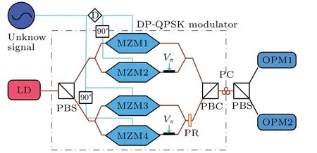
Fig. 1. Schematic diagram of instantaneous frequency measurement, LD:laser diode; PC: polarization controller; D: delay line; MZM: Mach-Zehnder modulator;PBC:polarization beam combiner;PR:polarization rotator;PBS:polarization beam splitter;OPM:optical power monitor.
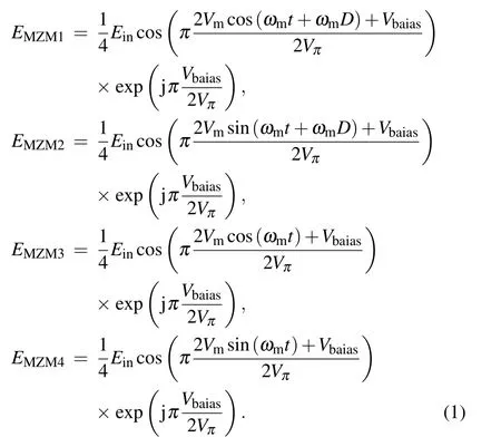
The optical field from the MZM1-MZM4 is given by
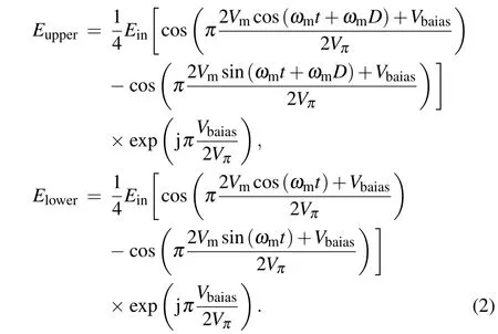
The optical field from the upper arm and lower arm can be written as
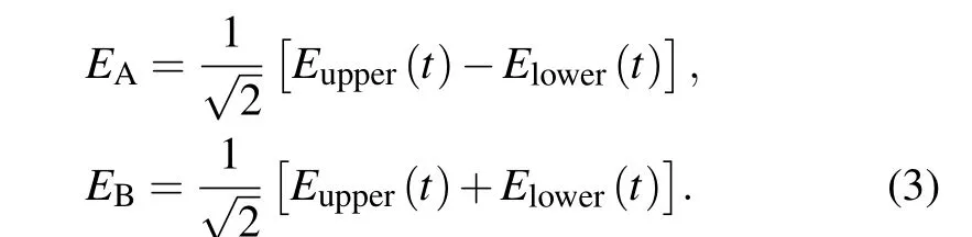
The modulated optical signals are combined by a polarization beam combiner(PBC).Then,the output signal from DPQPSK modulator is sent to a polarization beam splitter(PBS)via a PC.Here,the PC is used to align the output signal’s polarization direction at an angle of 45°with respect to the principal axis (EupperandElower) of PBS. The optical field at the output of PBS at port A and port B areEAandEBand can be expressed as follows:
The two optical power monitors are used to monitor the optical power after PBS.Through the ratio between the two measured power values, the amplitude comparison function (ACF) can be obtained. In this paper,the theoretical analyses of MZM1-MZM4 in different working conditions are carried out.
By adjusting the DC biases of the DP-QPSK modulator (MZM1-MZM4), the measurement range and resolution can be switched. The detailed theoretical analyses of different working conditions are conducted as follows.
Case A When MZM1-MZM4 work at the maximum transmission point(Vbaias=0 V),equation(2)can be rewritten as
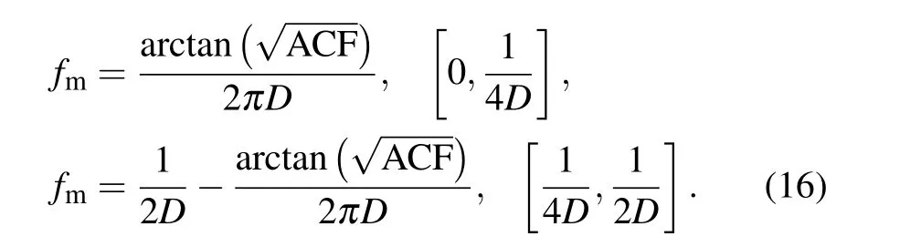
From Eqs. (7) and (11), the relationship between the optical power ratio and the frequency of unknown microwave signal is obtained. The formula of unknown microwave signal frequency can be obtained below.
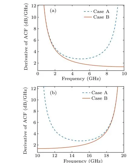
Fig. 2. The first-order derivatives of two ACFs in ranges of (a) 0 GHz-10 GHz and(b)10 GHz-20 GHz.
Thus,two methods can be used to achieve IFM in this system.Normally, the measurement range of IFM system is limited to the position of the first notch of the ACF in order to avoid frequency ambiguities. In our scheme, the notch point of the two cases is 1/4Dand 1/2D,respectively. The corresponding measurement range for the two cases can be obtained as

Then,the resolutions of the two cases are investigated. Since the measurement resolution is directly associated with the absolute value of slope of the ACF curve, in order to acquire a better comprehending of the performance improvement,the absolute values of the first-order derivatives of the ACFs for two cases are compared in 0 GHz-10 GHz and 10 GHz-20 GHz(D=25 ps)as shown in Fig.2.
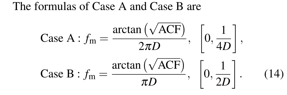
As can be seen in Figs.2(a)and 2(b), the absolute value of the first-order derivative of Case A is always higher than that of Case B,which means that Case A has a high resolution than Case B. The theoretically calculated ACF with respect toD=15, 20, 25, and 30 ps of two schemes are shown in Figs.3(a)and 3(b). It can be obtained that the notch point of Case A is 1/4Dand that of Case B is 1/2D. Obviously,Case A is more sensitive than Case B.
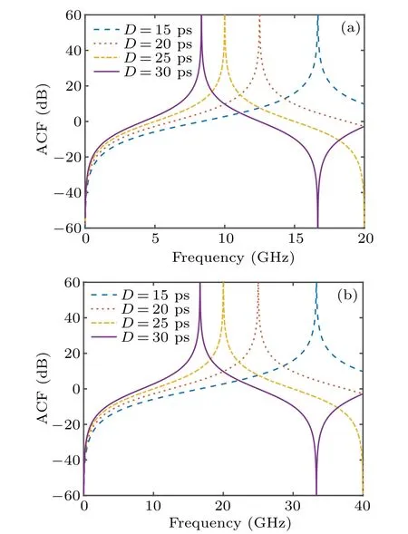
Fig.3. ACF curves of(a)Case A and(b)Case B at D=15 ps,20 ps,25 ps,and 30 ps.
According to the above theoretical analysis,a switchable IFM system is proposed. By settingVbaias=Vπ, the approximate range of the unknow RF signal can be obtained. ThenVbaiasis adjusted to 0 V to obtain more accurate measurement frequency. The instantaneous frequency can be calculated from the formula.
3. Simulation
To investigate its mechanism, simulations are preformed by using Optisystem 15.0. The setup is built up as shown in Fig. 1. The frequency of continue wave (CW) laser is 193.1 THz and the linewidth is 10 MHz. Then the laser is injected into a DP-QPSK modulator,which is designed by using a MATLAB program and a programmable module in Optisystem based on its characteristic. In the simulation of Case A,MZM1-MZM4 all work at the maximum transmission point(Vbaias=0 V)and MZM5 and MZM6 both work at the minimum transmission point(Vbaias=Vπ=4 V,Vπrepresents the half-wave switching voltage). The angle of the principal axis of the PBS with respect to DP-QPSK modulator should be 45°.Then,we use sinusoidal signal as an unknown signal to modulate the DP-QPSK modulator to verify the mechanism of the IFM system.
In order to investigate the laser power-independent characteristic of the scheme,we simulate the optical power curves under different power values of CW laser. By settingD=25 ps,figure 4(a)shows the optical power curves ofPAandPBunder power of CW laser of 0 dBm and 5 dBm, respectively.Obviously, the curves ofPAandPBare fully complementary and the difference value betweenPAandPBis identical for different laser power values. The notch points of the curves are both at 10 GHz, which is consistent with the theoretical result. Then by settingD=15, 20, 25, and 30 ps as shown in Fig. 4(b), the simulation results (symboled) are consistent with the theoretical results (line-denoted). It can be obtained that the measurement range is 16.7 GHz,12.5 GHz,10 GHz,and 8.3 GHz,respectively,which are consistent with the theoretical results. TakingD=25 ps for example,we compare the theoretical frequency (line-denoted) with the simulation frequency(symboled)as shown in Fig.4(c). The estimated error is shown in Fig.4(d). It can be obtained that estimated error is less than 80 MHz when the measurement range is in a range of 0 GHz-10 GHz,which apparently illustrates the validity of proposed IFM system.
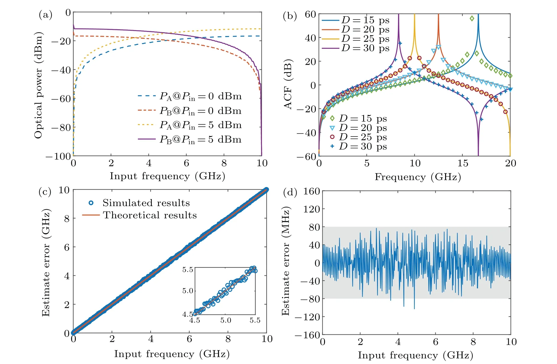
Fig.4. (a)Simulated curves of optical power(PA and PB)versus input frequency of Case A at D=25 ps and power values of CW laser P=5 dBm and 0 dBm. (b)Simulated and calculated curves of ACF of Case A at D=15,20,25,and 30 ps,with symbols marking simulated results and lines denoting calculated results. (c)Plots of measured frequency(symbol)and theoretical frequency(line)versus input frequency of Case A at D=25 ps. (d)Curve of estimated error versus frequency of Case A at D=25 ps.
Similarly, by adjusting the DC bias of each MZM(Vbaias=Vπ), Case B can be simulated and discussed. The optical power curves ofPAandPBat 0 dBm and 5 dBm, the simulated ACF curves and calculated ACF curves atD=15,20,25,and 30 ps as well as the estimated errors are also simulated. As shown in Fig.5(a),the notch points of the curves are all at 20 GHz,which accords well with the theoretical results.The ACF curves can be obtained when theDvalues are 15,20,25,and 30 ps as shown in Fig.5(b). The estimated error of the Case B is below 150 MHz and the measured results range from 0 GHz to 20 GHz as shown in Figs.5(c)and 5(d). It can be concluded that Case B has a larger measurement range and higher estimated error than Case A.
It is worth noting that there are four factors causing the estimated error in Figs. 4(d) and 5(d). Firstly, in order to simulate the possible influence of the actual environment,we add Gaussian white noise into the simulation. Secondly, the linewidth of the laser is 10 MHz, which will produce many low-order sidebands in the spectrum. Thirdly, the extinction ratio of MZM in the ideal state is infinite, which cannot be achieved in the simulation. Finally,owing to the limited storage space of computer,round-off error will also occur. However,in practice,the limitations induced by the imperfection of components and external environmental factors may also affect the measurable frequency range and accuracy of the proposed system. To optimize the parameter in simulated IFM system,In the following subsections four possible error factors will be discussed and their influences will also be analyzed.
Fig. 5. (a) Simulated curves of optical power (PA and PB) versus input frequency of Case B at D=25 ps and power of CW laser P=5 dBm and 0 dBm. (b)Simulated and calculated curves of ACF versus input frequency of Case B at D=15,20,25,and 30 ps,with symbols marking simulated results,and lines denoting calculated results. (c)Plots of measured frequency(marks)and theoretical frequency(line)versus input frequency of Case B at D=25 ps. (d)Curve of estimated error versus input frequency of Case B at D=25 ps.
3.1. Influence of polarization angle drift
In the proposed system, polarization angleαshould be maintained at 45°. In practice, the polarization angle may not exactly be at 45°because of the inaccuracy of the PC or external perturbation, which will weaken performance of the proposed IFM system. We take time delayD=25 ps for example to simulate the shifting of polarization angle. The polarization angle is assumed to be 45°+Δα(Δα=0°,±1°,±2°,±3°,±4°, and±5°), where Δαrepresents the polarization angle deviation. The ACF curves and the estimated error curves of Case A are shown in Figs. 6(a) and 6(b) and those of Case B are displayed in Figs. 7(a) and 7(b), respectively. To some extent, the absolute value of ACF curve decreases with the increase of polarization angle drift,especially in the boundary of measurement range, which are shown in Figs.6(a)and 7(a). The estimated errors are relatively large at 0 GHz and 10 GHz in Case A,which will increase to around±20 MHz,±200 MHz,±450 MHz,±700 MHz,±900 MHz,and±1.15 GHz at Δα=0°,±1°,±2°,±3°,±4°,and±5°as shown in Fig.6(b). To achieve high resolution(≤100 MHz)and relatively wide range,Δαis supposed to be limited in less than±3°, where the measurement range will be 0.5 GHz-9.5 GHz as shown in Fig. 6(b). As shown in Fig. 7(b), for Case B, the estimated error is relatively large at 0 GHz and 20 GHz,which will increase to around±20 MHz,±100 MHz,±200 MHz,±350 MHz,±450 MHz, and±550 MHz, at 0°,±1°,±2°,±3°,±4°, and±5°. Within the estimated error of 200 MHz, Δαshould be controlled carefully(Δα ≤±3°),where the measurement range will be 2 GHz-18 GHz as shown in Fig. 7(b). In order to improve the performance of the IFM system,a control circuit can be added to PC through feedback control to improve the accuracy of PC which is relatively expensive. To reduce cost,the polarization maintaining fiber patch cord with a specially designed connector key can be used to set at 45°to replace the PC.[17]
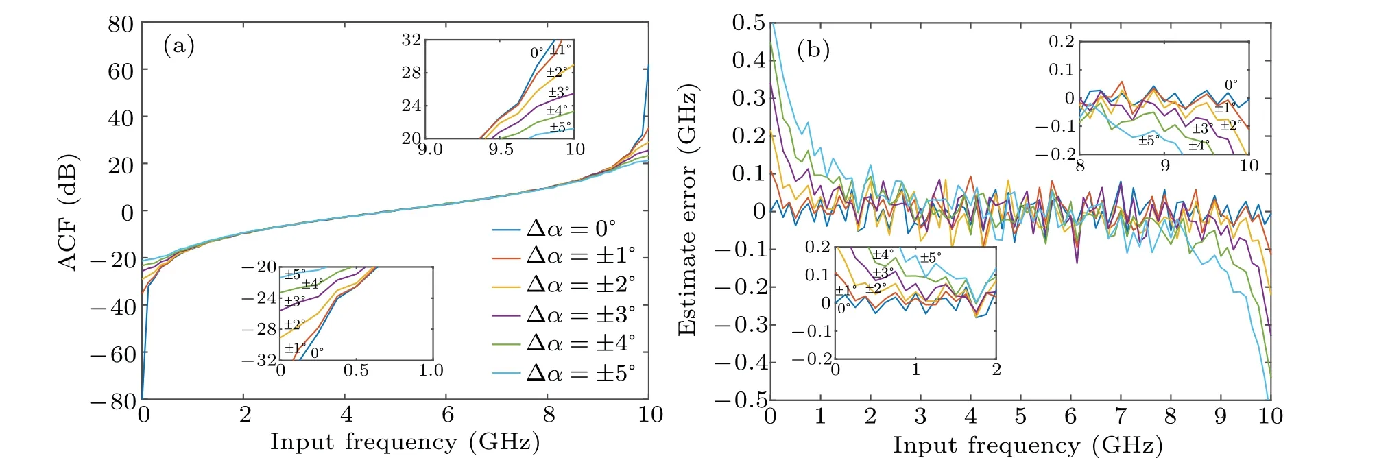
Fig.6. (a)Curves of ACF versus input frequency of Case B at Δα =0°,±1°,±2°,±3°,±4°,and±5° and at D=25 ps. (b)Curves of estimated error versus input frequency of Case A at Δα =0°,±1°,±2°,±3°,±4°,and±5° and at D=25 ps.
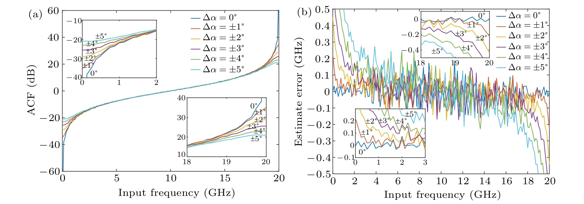
Fig.7. (a)Curves of ACF versus input frequency of Case B at Δα =0°,±1°,±2°,±3°,±4°,and±5° and at D=25 ps. (b)Curves of estimated error versus input frequency of Case B at Δα =0°,±1° ,±2°,±3°,±4°,and±5° and at D=25 ps.
3.2. Influence of voltage bias
The variation of external temperature will cause the bias voltage to drift, thereby affecting the ACF curve and narrowing the range of frequency measurement.The bias voltage drift is denoted as ΔVbaiasand the bias voltage of Case A and Case B are represented by ΔVbaiasandVbaias+ΔVbaiasrespectively.In Mach-Zehnder (MZ) modulator,Vbaiaswill be reflected in the output signal in the form of phase shift(φ1=πVbaias/Vπ),so the phase shift angle Δφ1can be used to indicate ΔVbaias(Δφ1=πΔVbaias/Vπ). The ACF curves and the estimated error of Case A is shown in Figs. 8(a) and 8(b), while Case B is shown in Figs. 9(a) and 9(b). As shown in Figs. 8(a) and 9(a), the absolute values of ACF curves decrease obviously around the boundary of measurement range. At Δφ1= 0°,±2°,±4°,±6°, and±8°, the estimated errors of Case A are about±20 MHz,±200 MHz,±550 MHz,±800 MHz,and±1.05 GHz at the boundary of range, which is shown in Fig. 8(b). The bias voltage can be easily controlled by the bias-voltage control circuit.
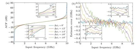
Fig. 8. (a) Curves of ACF versus input frequency of Case A at Δφ1 =0°, ±2°, ±4°, ±6°, and ±8° and at D=25 ps. (b) Curves of estimated error versus input frequency of Case A at Δφ1=0°,±2°,±4°,±6°,and±8° and at D=25 ps.

Fig. 9. (a) Curves of ACF versus input frequency of Case B at Δφ1 =0°, ±2°, ±4°, ±6°, and ±8° and at D=25 ps. (b) Curves of estimated error versus input frequency of Case B at Δφ1=0°,±2°,±4°,±6°,and±8° and at D=25 ps.
Within the estimated error below 100 MHz and by using bias-voltage control circuit (Δφ1≤4°), the measurement range is 1.5 GHz-8.5 GHz in Case A as shown in Fig. 8(b).When the values of Δφ1are 0°,±2°,±4°,±6°,and±8°,the estimated errors of Case B will reach to around±20 MHz,±150 MHz,±300 MHz,±450 MHz, and±500 MHz at the boundary of range,respectively,as shown in Fig.9(b). By using bias-voltage control circuit (Δφ1≤4°), the measurement range will be 1 GHz-19 GHz,when the resolution is relatively high (≤200 MHz). To suppress the drift of bias voltage, the voltage source can adopt a constant-voltage computerized numerical control(CNC)power supply,and the resolution of the current constant voltage CNC power supply can reach 0.001 V.In our system,the voltage offset less than 0.08 V can meet the system requirements, which means that the constant voltage CNC power supply can be applied to our system.
3.3. Influence of electrical delay line
The electric delay line may affect the measurement range of the IFM system,due to inaccurate delay and microwave signal power attenuation. Aiming at these two effects, the ACF curves and estimated error of the frequency measurement system are simulated and analyzed.
Owing to the limited resolution of the delay line,the time delay may deviate from the expected value. We assume that the time drift is Δτ. The simulation of the IFM system is conducted separately at Δτ=0 ps, 0.2 ps, and 0.3 ps is given when we expectD=25 ps. Figures 10(a) and 10(b) display the ACF curves and estimated error of Case A, respectively.Meanwhile,figures 11(a)and 11(b)show the ACF curves and estimated error of Case B.It can be obtained that in Fig.10(a),the ACF curve deviates to the left or right around 10 GHz with the increase or decrease of time delay. Theoretically,the amplitude of ACF curve will not change. However, owing to the selection of sampling points,the amplitude of ACF curve changes.With high resolution(estimated error≤100 MHz)of Case A,the delay deviation should be within 0.2 ps as shown in Fig. 10(b). Around 20 GHz, ACF curves of Case B shift with the change of time delay as shown in Fig.11(a). The delay deviation should also be within 0.2 ps with estimated error less than 200 MHz as shown in Fig.11(b).It can be concluded that the time delay of our proposed system should be carefully controlled. However,the time delay of tunable delay line cannot be accurately calibrated. In our proposed IFM system,electrical cable can be used to introduced fixed time delay. By adjusting working state of DP-QPSK modulator, high resolution in an appropriate measurement range can be achieved.
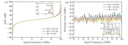
Fig.10. (a)Curves of ACF versus input frequency of Case A at Δτ =0.3 ps,0.2 ps,and 0 ps at D=25 ps. (b)Curves of estimated error versus input frequency of Case A at Δτ =0.3 ps,0.2 ps,and 0 ps at D=25 ps.

Fig.11. (a)Curves of ACF versus input frequency of Case B at Δτ =0.3 ps,0.2 ps,and 0 ps at D=25 ps. (b)Curves of estimated error versus input frequency of Case A at Δτ =0.3 ps,0.2 ps,and 0 ps at D=25 ps.

Fig.12. (a)Curves of ACF versus input frequency of Case A at L=0 dB,0.2 dB,0.4 dB,0.6 dB,0.8 dB,and 1 dB and at D=25 ps. (b)Curves of estimated error versus input frequency of Case A at L=0 dB,0.2 dB,0.4 dB,0.6 dB,0.8 dB,1 dB and at D=25 ps.

Fig.13. (a)Curves of ACF versus input frequency of Case B at L=0 dB,0.2 dB,0.4 dB,0.6 dB,0.8 dB,and 1 dB and at D=25 ps. (b)Curves of estimated error versus input frequency of Case B at L=0 dB,0.2 dB,0.4 dB,0.6 dB,0.8 dB,and 1 dB and at D=25 ps.
At the same time, the electric delay line will also cause the power of microwave signal to attenuate. The effect on signal power increases with microwave frequency increasing.When the microwave signal is at 20 GHz, the loss is within 1 dB.By setting the loss of microwave signal to beL,the simulations of the ACF curve and the estimated error are given whereL=0 dB, 0.2 dB, 0.4 dB, 0.6 dB, 0.8 dB, 1 dB, andD=25 ps. The ACF curve and estimated error of Case A are shown in Figs.12(a)and 12(b),and those of Case B are shown in Figs.13(a)and 13(b).With the increase of the loss,the ACF curve tends to be flat at both ends of 0 GHz and 10 GHz as shown in Fig.12(a). WhenL=1 dB,the measurement range of Case A is from 2 GHz to 8 GHz with estimate error less than 0.1 GHz as shown in Fig.12(b). The trends of ACF curves of Case B are the same at the boundary of measurement range as shown in Fig.13(a). The measurement range of Case B is from 1 GHz to 19 GHz with estimate error less than 0.2 GHz as shown in Fig. 13(b). It can be obtained from the above analysis that our proposed system can cope with the influence resulting from the increase of delay line loss with the increase of microwave signal frequency.
3.4. Influence of chirp
There are two sources of chirp in the proposed system,which are the drive signals applied to phase modulator and the finite extinction ratio of the MZM. The influence of modulator chirp effect on frequency measurement system is simulated and analyzed.
In the proposed system, four 180°hybrid couplers will be used to realize push-pull operation. In practice, owing to the component imperfection, there will happen a phase drift in hybrid coupler which will introduce the chirp into MZM.Thus, the influence of hybrid phase balance should be discussed. For example, the electrical time delay is also set to beD=25 ps. The four couplers are identical and the phase drift is Δβ. Therefore, the phase difference between two RF ports of each MZM is 180°+Δβ. We simulate the ACF curve and the estimated error Δβ=0°,±2°,±4°,±6°, and±8°.The ACF curves and the estimated error curves of Case A are displayed in Figs. 14(a) and 14(b) and those of Case B are displayed in Figs. 15(a) and 15(b). As shown in Figs. 14(a)and 15(a),the ACF curves decrease distinctly around 10 GHz and 20 GHz, respectively, of Case A and Case B. As shown in Fig. 14(b), around 10 GHz, the estimated error of Case A will reach to 20 MHz, 200 MHz, 600 MHz, 800 MHz,and 1.1 GHz, respectively, at Δβ=0°,±2°,±4°,±6°,±8°.To guarantee that the accuracy of estimated error is less than 100 MHz and the measurement range is relatively feasible,the phase drift should be controlled to be within 4°as shown in Fig.14(b). In that case,the measurement range of Case A will be 0 GHz-8.5 GHz. Around 20 GHz, the estimated errors of Case B will turn to be around 20 MHz, 100 MHz, 250 MHz,400 MHz,and 500 MHz,respectively,at Δβ=0°,±2°,±4°,±6°,and±8°as shown in Fig.15(b). For high resolution and relatively feasible measurement range, the phase drift should be controlled to be within 8°,where the measurement range is 0 GHz-19 GHz as shown in Fig.15(b). The influence of hybrid phase balance can be reduced by precise control,a delay and power tunning component can be added into the input of lower arm to improve the performance.[17]
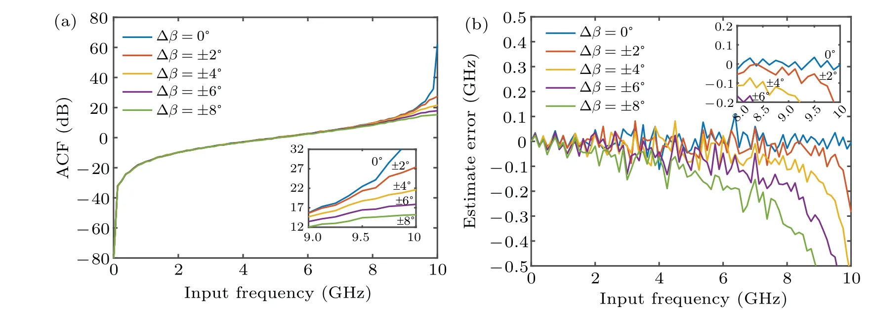
Fig.14. (a)Curves of ACF input frequency of Case A at Δβ =0°, ±2°, ±4°, ±6°, and±8° and at D=25 ps. (b)Curves of estimated error versus input frequency of Case A at Δβ =0°,±2°,±4°,±6°,and±8° and at D=25 ps.
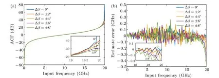
Fig.15. (a) Curves of ACF versus input frequency of Case B at Δβ =0°, ±2°, ±4°, ±6°, and±8° and at D=25 ps. (b)Curves of estimated error versus input frequency of Case B at Δβ =0°,±2°,±4°,±6°,and±8° and at D=25 ps.
Extinction ratio is determined by the properties of modulators which is expect to be infinite. In practice, the finite extinction ratio will cause the optical signal to chip in the system and then make an influence on frequency measurement. The ER represents the value of extinction ratio of IFM.The ACF curves and estimated error of Case A atD=25 ps,ER=40 dB,35 dB,30 dB,25 dB are shown in Figs.16(a)and 16(b),respectively. The peaks of ACF curves decrease around 10 GHz as ER decreases, and estimate errors are around 150 MHz, 300 MHz, 500 MHz, 850 MHz, at ER=40 dB,35 dB,30 dB,25 dB,respectively,as shown in Figs.16(a)and 16(b).To achieve the high resolution(≤100 MHz),the extinction ratio should be above 30 dB and the measurement is in a range from 0 GHz to 9 GHz. Figures 17(a) and 17(b) show the ACF curves and estimated error of Case B, respectively.As shown in Fig. 17(a), the peaks of ACF curves decrease around 20 GHz as ER decreases. The estimated errors are below 200 MHz at ER=40 dB,35 dB,30 dB,25 dB as shown in Fig. 17(b), which means high resolution (≤200 MHz) of Case B can be achieved when ER is above 25 dB.Fortunately,the ER of commercial MZM can reach more than 30 dB.
In this subsection, the theoretical part is verified by simulation. Besides,four possible factors of the inaccuracy of the components in this system are discussed,they being the polarization angle of PBS,the DC bias,the chirp of MZM,and the electrical delay line. The corresponding measures to improve the components performance have been described after analysis, thereby the estimated errors of both Case A and Case B can be restricted in an acceptable boundary (≤100 MHz,≤200 MHz).
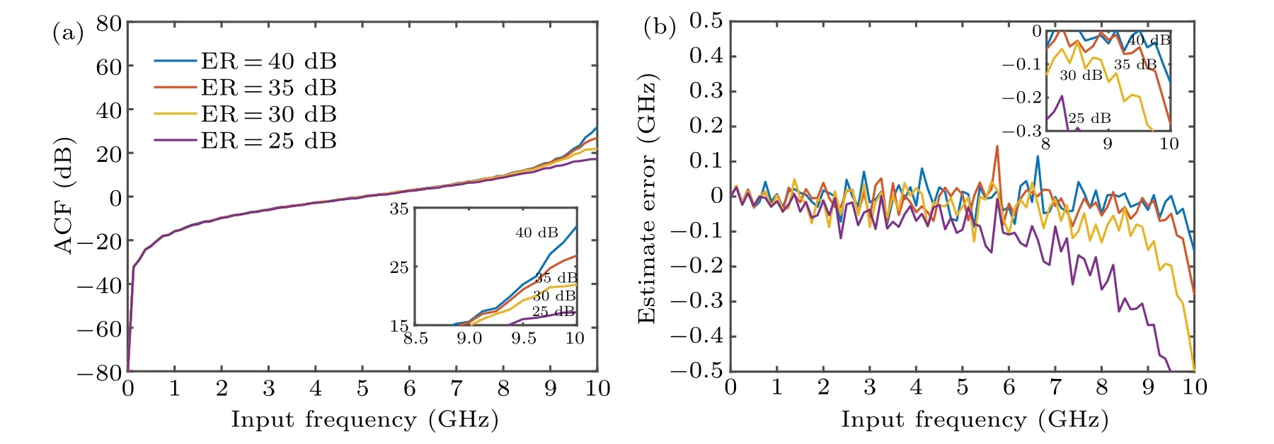
Fig.16. (a)Curves of ACF versus input frequency of Case A at ER=40 dB,35 dB,30 dB,and 25 dB and at D=25 ps. (b)Curves of estimated error versus input frequency of Case A at ER=40 dB,35 dB,30 dB,and 25 dB and at D=25 ps.
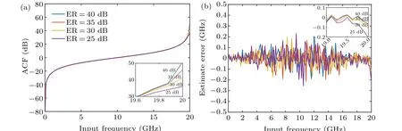
Fig.17. (a)Curves of ACF versus input frequency of Case B at ER=40 dB,35 dB,30 dB,and 25 dB and at D=25 ps. (b)Curves of estimated error versus input frequency of Case B at ER=40 dB,35 dB,30 dB,and 25 dB and at D=25 ps.
It is worthy to note that for most of IFM cases,there exists the trade-off issue between the measurement range and resolution,which means that the measurement range needs to be sacrificed in order to obtain a high resolution. In practical applications,a two-step measurement based our proposed scheme can be used to solve this problem.Firstly,as illustrated in Case B,by settingVbaias=Vπ,the IFM with relatively large range(-1/2D)is achieved from Eq.(13). If the measurement range is divided into two regions including-1/4Dand 1/4D-1/2D,the frequency region of unknown microwave signal can be estimated. Next, by adjustingVbaiasto 0 V, the IFM with relatively high resolution as shown in Case A is realized. Owing to the symmetry of ACF curve,the measurement range in this case a can be extended to 0 GHz-1/2DGHz. The corresponding formula in this step is
Since we can obtain the rough frequency region of the unknown signal from the first step,according to Eq.(18),the more accurate measurement can be achieved. That is to say,the frequency measurement range of the system can reach to 1/2D,which is determined through the first step,and then the signal frequency can be measured more accurately through the second step. Thus,our proposed switchable IFM method can solve the trade-off problem and may find applications in future low-cost IFM with both high resolution and large measurement range.
4. Conclusions
In this work,we have proposed an IFM system based on power monitoring by using DP-QPSK modulator. By simply adjusting the DC biases of the DP-QPSK modulator instead of changing the electrical delay,the measurement range and resolution of the system can be switched.The theoretical analysis and the simulation of the IFM system are conducted to display and verify the mechanism. We takeD=25 ps for example,by adjusting the DC biases fromVπto 0 V, the measurement range can be extended from 0 GHz-20 GHz to 0 GHz-10 GHz and the resolution can be switched from 150 MHz to 80 MHz.Since the imperfect property of devices may affect the feature of the proposed system, four possible factors of the inaccuracy of the components are discussed,including the polarization angle of PBS, the DC bias of MZM, the chirp of MZM,and the electrical time delay line. It is found that the estimated errors of the system can be limited in an acceptable boundary(≤100 MHz) when the property of polarization angle drift,phase shifter and DC bias can be controlled (polarization angle of PC Δα ≤±3°, phase balance of the MZM Δβ ≤±4°,extinction ratio of the MZM ER≥30 dB, DC bias of MZM Δφ1≤±4°,delay deviation of TDL Δτ ≤0.2 ps). Compared with the existing IFM method,the optical filter or the high frequency PD is no longer needed in the proposed scheme,which means that the resolution can be higher since it can avoid the measuring error induced by wavelength drifting,electrical noise,and EMI.Besides,the switchable characteristic and no high frequency electrical devices can further increase the flexibility and reduce the cost. Thus,we believe that the proposed architecture can provide a cost-effective and flexible solution for future dynamic microwave frequency measurement.
Acknowledgements
Project supported by the National Natural Science Foundation of China(Grant No.61801017,U2006217,62005011,and 61620106014),Beijing Municipal Natural Science Foundation (Grant No. 4212009) and the Fundamental Research Funds for the Central Universities(Grant No.2020JBM010).
猜你喜欢
现代苏州(2022年9期)2022-05-26
红蜻蜓·低年级(2022年5期)2022-05-25
青年文学家(2021年31期)2021-12-12
少先队活动(2021年9期)2021-11-05
医学食疗与健康(2021年27期)2021-05-13
照相机(2021年2期)2021-04-06
考试与评价·高二版(2020年3期)2020-09-10
青年文学家(2020年16期)2020-07-13
学生天地(2019年36期)2019-08-25
作文世界(小学版)(2018年10期)2018-11-13

- Chinese Physics B的其它文章
- Quantum walk search algorithm for multi-objective searching with iteration auto-controlling on hypercube
- Protecting geometric quantum discord via partially collapsing measurements of two qubits in multiple bosonic reservoirs
- Manipulating vortices in F =2 Bose-Einstein condensates through magnetic field and spin-orbit coupling
- Beating standard quantum limit via two-axis magnetic susceptibility measurement
- Neural-mechanism-driven image block encryption algorithm incorporating a hyperchaotic system and cloud model
- Anti-function solution of uniaxial anisotropic Stoner-Wohlfarth model