Exact solutions of the Schr¨odinger equation for a class of hyperbolic potential well

Xiao-Hua Wang(王晓华) Chang-Yuan Chen(陈昌远) Yuan You(尤源)Fa-Lin Lu(陆法林) Dong-Sheng Sun(孙东升) and Shi-Hai Dong(董世海)

1School of Physics and Electronic Engineering,Yancheng Teachers University,Yancheng 224007,China

2Research Center for Quantum Physics,Huzhou University,Huzhou 313000,China

3Laboratorio de Informaci´on Cu´antica,CIDETEC,Instituto Polit´ecnico Nacional,UPALM,C.P 07700,CDMX,Mexico

Keywords: hyperbolic potential well,Schr¨odinger equation,Wronskian determinant,confluent Heun function

1. Introduction

As we know, one of the fundamental tasks of quantum mechanics is to explore the exact solution of the Schr¨odinger equation for all kinds of potential fields by using different methods.[1-3]Because the hyperbolic potential well has important applications in physics,[4-8]the symmetric and asymmetric single and double-well shapes have been studied widely by many methods,such as asymptotic iteration method(AIM),Bethe ansatz method, and the confluent Heun function approach that can be broken into anNdegree polynomial under certain constraints,etc.[9-23]It should be emphasized that these methods focus on how to obtain more accurate eigenvalues but pay less attention to explicit eigenfunctions except for the modified P¨oschl-Teller potential.[24-26]

The parametersuandLdenote the depth and width of potential wellUq(x;u,L)respectively,anduis a dimensionless parameter. For these potential wells,only in Ref.[13]AIM was used to study the eigenvalue of potential wellU2,and the other two have never been reported to our best knowledge.Taking a simple change of variablex＇=x/Ltransforms equation(1)into a single parameter Schr¨odinger equation

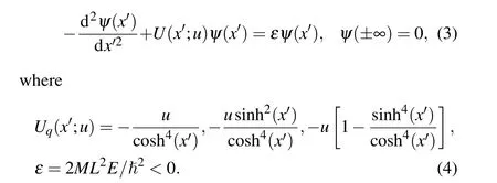
We notice thatUq(x＇;u) is an even function without singularity as illustrated in Fig. 1. On the other hand, it is found that theU1,3are both single well with potential depthu, andU2is a double well with potential depthu/4. Referring to Refs. [1-3,27,28], the number of bound states is finite for the potential wellUq. No matter how shallow the potential well is, there exists at least one even parity bound state.According to the basic principles of quantum mechanics, the bound state is non-degenerate and the eigenfunction satisfiesψn(-x＇)=(-1)nψn(x＇), wherenis the number of the nodes of the wave function.

This paper is organized as follows: In Section 2 based on our recent works,[29-33]takingU1as a typical example,we describe how to accurately solve the bound states of the Schr¨odinger equation. For this purpose, the first step is to transform the corresponding Schr¨odinger equation into a confluent Heun differential equation by using different forms of variable substitution and function transformation and then obtain two linearly dependent solutions for the same eigenstate.The second step is to construct a Wronskian determinant from those two linearly dependent solutions and then based on it to obtain an energy spectrum equation. As a result,the quantum number corresponding to each eigenstate and the total number of bound states can be illustrated graphically through studying this energy equation. The third step is to calculate the exact energyεof each eigenstate with the aid of Maple. Finally,by substituting the obtained energyεinto the wave function we are able to get the explicit wave function expressed by the confluent Heun function and also study their linear correlation. In Sections 3 and 4,the exact solutions of potential wellsU2andU3are investigated briefly in a similar way. The conclusions of this paper are finally given in Section 5.

Fig.1. The plot of the hyperbolic potential wells with two different depth u.

2. Exact solutions of potential well U1

We notice that both equations (14) and (19) are solutions to the differential equation(7). This is a typical Sturm-Liouville problem,i.e.,the eigenvalues are the real numbers;the eigenstates are not degenerate and the eigenfunctions will form an orthonormalized complete set. Thus,these two eigenfunctions belonging to the same eigenstate except for having different mathematical expressions should be convergent for the same eigenvalueεaty=±1(x＇ →±∞) and must also be linearly dependent within the intervaly ∈(-1,1).[37-39]For two nonzero constantsC1andC2, the solutions of Eq. (7) has the relationC1ψ1(x＇)+C2ψ2(x＇)=0. Substitution of Eqs.(14)and(19)into it leads toC1F(1)+C2F(2)=0,whose first derivativeC1F＇(1)+C2F＇(2)=0. From these two relations we obtain a useful Wronskian determinant

Fig.2. Plot of Re f(ε)as a function of ε with different depths u for the potential well U1.

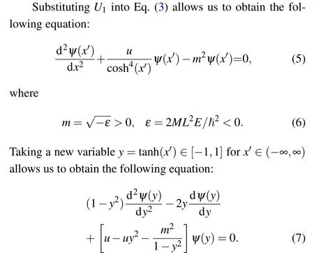
Table 1. Precise values of the dimensionless energy ε for the potential well U1.

For-u ＜ε ＜0,the intersection of the function Ref(ε)with the‘εaxis’is nothing but the definite eigenvalue. For a givenu,the number of intersection to‘εaxis’is finite,which corresponds to the number of bound states (see Fig. 2). For example,only one bound state exists foru=0.01 and 1,two bound states foru= 5 and 10, while six bound states foru=100,etc. As a convention,the leftmost intersection is the ground state with the lowest energy(i.e.n=0), the next followed intersection is the first excited state with the quantum numbern=1. From Eq. (22), the precise values of corresponding quantum numbernand energyεfor different depthucan be calculated by using Maple, the results are listed in Table 1.

Before ending this part,let us study the linear dependence between these two eigenfunctions as displayed in Fig.3.Since both equations(14)and(19)are complex functions, after the calculated eigenvalues are substituted into them, we find that their real and imaginary parts have the following relations:

As what follows, we are ready to study other two potential wellsU2,3as the case ofU1.

Fig. 3. Linear dependence between complex eigenfunctions ψ1(x/L) and ψ2(x/L)for the potential well U1(u=10). (a)Real part for n=0,(b)imaginary part for n=0,(c)real part for n=1,(d)imaginary part for n=1.

3. Exact solutions of potential well U2

After substitutingU2into Eq. (3) and taking the same variabley,we may rewrite Eq.(3)as

determine the accurate eigenvaluesεand the number of bound states. Studying Eq. (29) enables us to decide how many the bound states have(i.e.quantum numbern)and the precise energyεby using Maple. The results given in Table 2 are exactly same as those of Ref.[13]. Moreover,after substituting the calculated eigenvalues into Eq. (27) to perform the normalization operation, we find the following relation between them

which implies that they are linearly dependent(see Fig.5).

Fig.4. Plot of f(ε)as a function of ε with different depth u for the potential well U2.

Table 2. Precise values of the dimensionless energy ε for potential well U2.

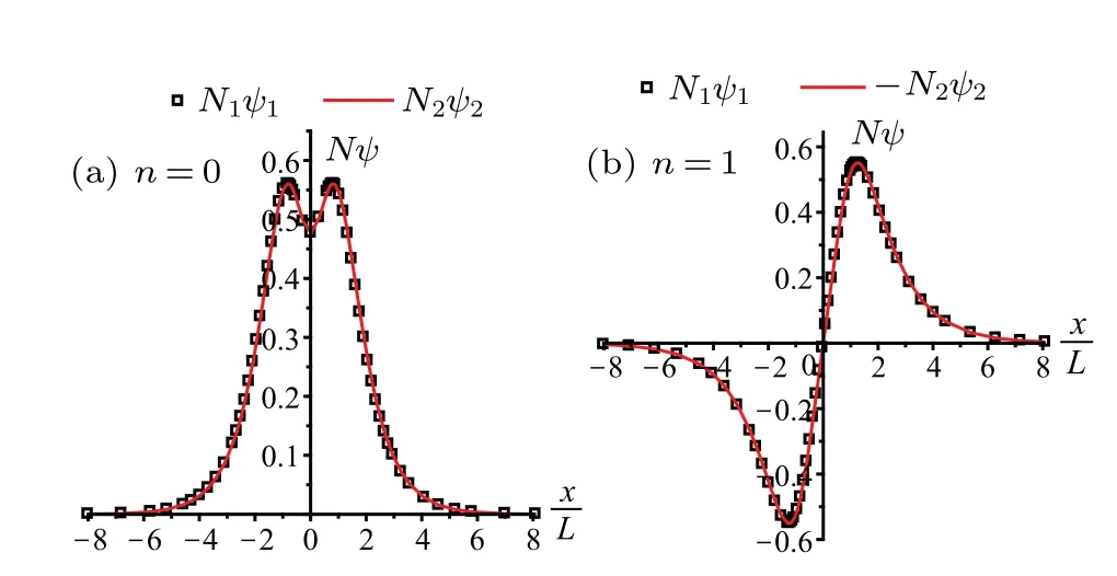
Fig. 5. Linear dependence between real eigenfunctions ψ1(x/L) and ψ2(x/L)for the potential well U2(u=10).

4. Exact solutions of potential well U3

In a similar way to above, the corresponding Eq. (3) in this case becomes

The corresponding two linearly dependent solutions for this potential well are given by

to show its intersections with‘εaxis’for different depthuas illustrated in Fig. 6. The results are listed in Table 3. After substituting the eigenvalues,which is calculated by solvingf(ε)=0,into Eq.(32),we find they satisfy the relation(30),which implies that they are linearly dependent as displayed in Fig.7.

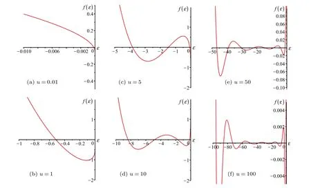
Fig.6. Plot of f(ε)as a function of ε with different depth u for the potential well U3.

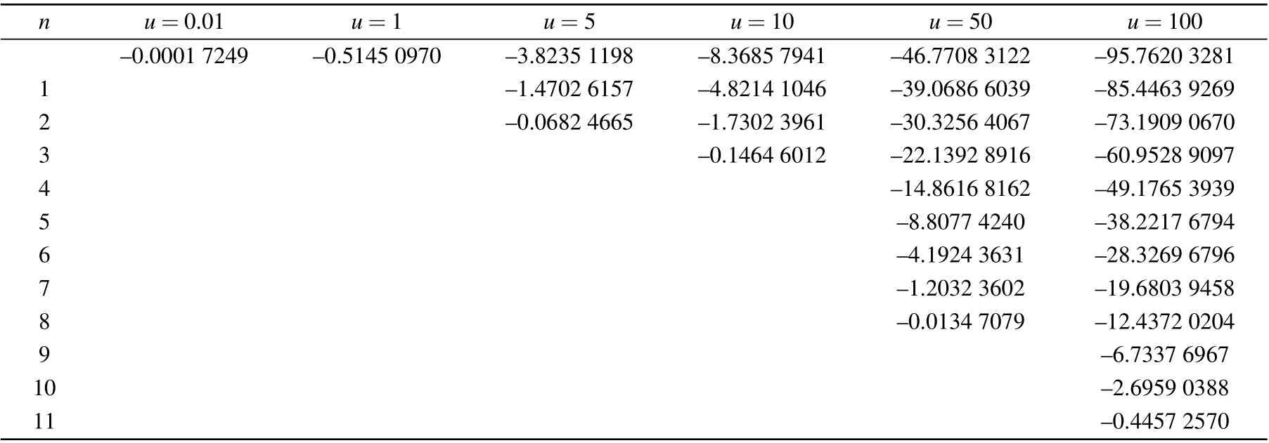
Table 3. Precise values of the dimensionless energy ε for the potential well U3.

Fig.7. Linear dependence between real eigenfunctions ψ1(x/L)and ψ2(x/L)for the potential well U3(u=10).

5. Conclusion

In this paper following the method used in our previous works,[29-33]we explored the exact solutions of the Schr¨odinger equation for a class of hyperbolic potential wells.This was realized by transforming the Schr¨odinger equation into a confluent Heun differential equation through using different forms of variable substitution and function transformation. And then two linearly dependent solutions for the same eigenstates were found to be used for constructing a Wronskian determinant, which leads to the energy spectrum equation. Then,the quantum number corresponding to each eigenstate and the total number of bound states are graphically displayed.After that,we used Maple to calculate the exact energyεof each eigenstate for different potential wellUq.Finally,the analytical wave function expressed by confluent Heun function can be gotten by substituting the obtained energy into the wave function.Before ending this work,we give two useful remarks on this method. In Ref.[15],when studying the hyperbolic potential well,the confluent Heun function satisfies two constraints,[15,34-36](i)ΔN+1(µ)=0,and(ii)µ+ν+Nα=0.The confluent Heun function will be truncated into anNdegree polynomial to obtain the energy and the analytical wave function under special conditions. It is obvious to have some limitations to such an approach. This is because the second constraint (ii) cannot be satisfied for the present problem according to Eq.(11). As a result,the class of hyperbolic potential well studied here cannot be treated by the current method.It should be pointed out that the present method is especially suitable for symmetric regions with no singular points and no degeneracy of the eigenstates. In addition, the calculation of related functions in Maple may be not efficient for some special values, especially large parameters. We expect that this shortcoming will be improved as the version of Maple is updated.

Acknowledgements

Project supported by the National Natural Science Foundation of China (Grant No. 11975196) and partially by SIP, Instituto Polit´ecnico Nacional (IPN), Mexico (Grant No. 20210414). Prof. Dong started this work on Sabbatical Leave of IPN.