Solving quantum rotor model with different Monte Carlo techniques

Weilun Jiang(姜伟伦) Gaopei Pan(潘高培) Yuzhi Liu(刘毓智) and Zi-Yang Meng(孟子杨)

1Beijing National Laboratory for Condensed Matter Physics and Institute of Physics,Chinese Academy of Sciences,Beijing 100190,China

2School of Physical Sciences,University of Chinese Academy of Sciences,Beijing 100190,China

3Department of Physics and HKU-UCAS Joint Institute of Theoretical and Computational Physics,

The University of Hong Kong,Pokfulam Road,Hong Kong,China

4Songshan Lake Materials Laboratory,Dongguan 523808,China

Keywords: Monte Carlo methods

1. Introduction

The study of the critical behavior inXYmodel dates back to the early stage of renormalization group.[1]To date, very accurate analytical and numerical calculations at the (2+1)d O(2) Wilson-Fisher quantum critical point exist with high precision of exponents determined,[2-9]and the rich physics of such transition related with the superconductor-insulator,[10,11]superfluid-insulator[12,13]and easy-plane quantum magnetic[14]transitions have been well acknowledged by the community. Moreover, the presence of Kosterlitz-Thouless(KT)transition at finite temperature also illustrates the nontrivial topological character of the setting and the associated vortex excitations are appearing in various material realizations.[15-17]In short,the quantumXYcriticality and KT physics originated from the(2+1)d O(2)transition are rich and profound.

With the acknowledgement of its importance, the renormalization group expansion calculations have been performed upon the (2+1)d O(2) Wilson-Fisher fixed point and comparisons with the unbiased Monte Carlo simulation results are achieved,[7,8]lately conformal bootstrap calculation has also been succeeded in (2+1)d O(2) QCP.[9]Among different Monte Carlo simulation methods,such as local Metropolis,[2]Swendsen-Wang and Wolff-cluster,[18,19]over-relaxation,[20]worm-algorithm in the path-integral formalism,[6,21]etc, accurate results have also been obtained. The remaining issue is that there still lacks systematic analysis and comparison of the performance of various Monte Carlo schemes,both in terms of the autocorrelation time and physical CPU hours in achieving the same level of numerical accuracy. In this work,we would like to fill in this gap.

We implement the Monte Carlo simulation for (2+1)d quantum rotor model and focus on the performance of simulation in the vicinity of the(2+1)dXYquantum critical point.Among the five different update schemes we tested in this work,which are comprised of local Metropolis(LM),LM plus over-relaxation(OR),Wolff-cluster(WC),hybrid Monte Carlo(HM),hybrid Monte Carlo with Fourier acceleration(FA),we find that to achieve the same level of numerical accuracy of the physics observables at the(2+1)d O(2)QCP,the WC and FA schemes have the smallest autocorrelation time and cost the least amount of CPU hours. Moreover, since FA scheme is more versatile in terms of implementation for complicated Hamiltonians, it has the advantage towards the future development of the quantum many-body simulations in which the simulation of O(2)lattice boson is the central ingredient.

For example, the Fermi surface Yukawa-coupled to critical O(2) bosons at (2+1)d will be the natural extension of the system of Fermi surface Yukawa-coupled to critical Ising bosons where concrete numerical evidences of the non-Fermi-liquid[22,23]and quantum critical scaling beyond the Hertz-Mills-Moriya framework[23]have been revealed recently. Also, when the gauge field with U(1) symmetry couples to matter field at (2+1)d, such as the Dirac fermion in the recent case,[24,25]although attempt succeeded in reaching small to large system sizes and established the existence of the U(1) deconfined phase even if the fermion flavor is justNf=2,[24]larger system sizes are inevitably crucial to further confirm such important discovery at the thermodynamic limit. Of course,the Monte Carlo simulation of these systems involves the update of fermionic determinant and therefore their computational complexity also comes from the fermionic part of the configurational weight,[26]the overall bottleneck can be overcome by finding an efficient update scheme of the U(1) (O(2)) gauge (boson) fields on the lattice upon the lowenergy effective model extracted from methods such as the self-learning approach.[27-29]These effective models usually acquire long-range interactions beyond the bare bosonic ones in the original Hamiltonian, and are difficult to handle with conventional methods such LM and WC discussed here.

Also,theXYand KT-related physics appear in several recently discovered frustrated magnets, such as the compound of TmMgGaO4,which nicely develops a Kosterlitz-Thouless melting of magnetic order in a triangular quantum Ising model setting.[15-17]One could certainly envision the application of different Monte Carlo schemes tested here to perform better simulation upon future models of quantumXYmagnets.

We end the introduction by briefly outline the structure of the paper. In Section 2, we describe the quantum rotor model and setup its path-integral formulation upon which the quantum Monte Carlo simulation will be carried out. In Section 3, we explain the different Monte Carlo update schemes employed in this work,and pay more attention to the HM and FA schemes which are less used in a condensed matter setting.Then Section 4 offers the results and compares the autocorrelation time and CPU hours of these methods at the (2+1)d O(2) QCP in details. Section 5 summarizes the main results and elaborates more on the relevance of this work towards to more frontier models in which the successful simulation of the quantum rotor model is of vital importance.

2. Model

We begin the discussion with the 2d Bose-Hubbard model on square lattice[2,10]

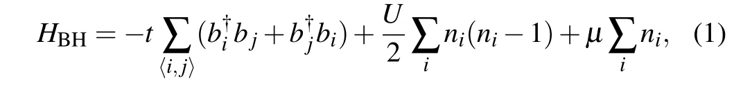
wheretis the nearest-neighbor hopping strength of boson,µis the chemical potential, andUis the on-site repulsion. The creation and annihilation operators of boson satisfy commutation relation[bi,b†j]=δi,jwhereδis the Kronecker function.At a fixed chemical potential, Eq. (1) describes the quantum phase transition from superfluid to Mott insulator as a function ofU/t. If the average filling of boson is an integer, then the transition is of(2+1)d O(2)universality with the dynamical exponentz=1,and if the average boson filling is deviated from integer,the transition is of(2+2)d O(2)universality with the dynamical exponentz=2.[10,12]In the former case, one can writebias|bi|eiθiand integrate out the amplitude fluctuations. Then the BH model becomes a model of coupled Josephson junctions,[12]

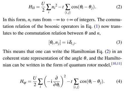
The derivative∂/∂θplays the role of angular momentum and can be further expressed in a path integral of the coherent state such that its Monte Carlo simulation becomes possible.We illustrative this process starting from the partition function

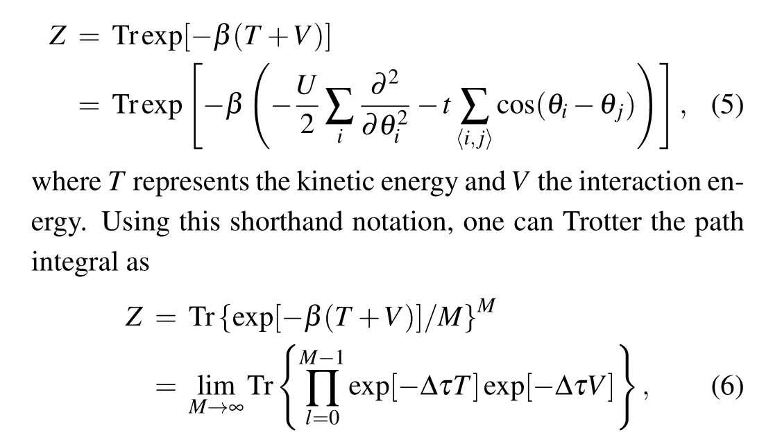
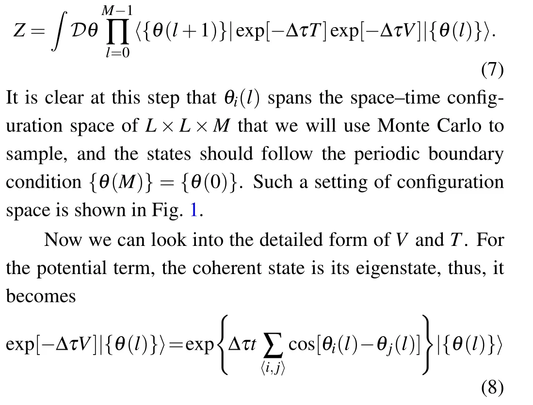
where the imaginary timeβhas been divide intoMslices with step Δτ=β/Mand we index the time slices with labell ∈[0,M-1]. Now one can insert the complete sets of the coherent state of{θ(l)}at each imaginary time step in Eq.(6)and have

From here on one can have two ways to simulate Eq.(12).One is by integrating out the variable{θi(l)}and arrives at a link model with integer-valued{Ji(l)}on every bond. This type of algorithm is not the main focus of this paper and we discuss it in Appendix A.

Fig.1. Schematic plot of the configuration space for the(2+1)d O(2)XY QCP.The blue arrows in the space-time coordinate stand for the unit vector{θi(l)} (or {θr} with r the space-time coordinate) in our simulation and the Kτ and Kx are the anisotropic temporal and spatial interaction strengths in the path-integral of Eq. (15). Along the axis of U/t, quantum critical point gc =(U/t)c separates the superfluid phase with O(2) XY symmetrybreaking and the disordered phase where the system is in a trivial and symmetric state.

3. Algorithm

The quantum rotor model in Eqs.(2),(12)and(15)can be solved with various Monte Carlo simulation schemes,including the local Metropolis (LM),[31]LM plus over-relaxation(OR),[5,20]Wolff-cluster(WC),[19]hybrid Monte Carlo(HM)and hybrid Monte Carlo supplemented with Fourier acceleration(FA).[32]In this section,we will elucidate the basic steps in these schemes with the detailed explanation in HM[33-35]and FA[36]schemes as they are more used in the high-energy community and less so to condensed matter.

3.1. Local update

This is the standard Monte Carlo update scheme,based on the Metropolis-Hastings algorithm.[31,37]In the rotor model setting, the update is comprised of the following steps: first we randomly choose one site,and then try to change theθi(l)by a random value within 0 to 2π. The acceptance of such update is determined by the Metropolis acceptance ratio. To satisfy ergodicity, we choose the site with its lattice index in sequence and define one Monte Carlo update step as a sweeping over the entire space-time configuration when calculating the autocorrelation time.

3.2. Over-relaxation update

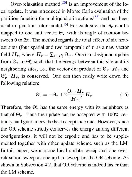
3.3. Cluster update

Here we employ the Wolff update scheme,it is one of the effective cluster update methods.[19]Since our model isXYmodel with O(2)symmetry,we can easily construct the global Wolff cluster. The basic principle is to grow a cluster with certain probability and change all of the sites in the cluster.For our model, we choose a random site at first and grow the cluster with the probability

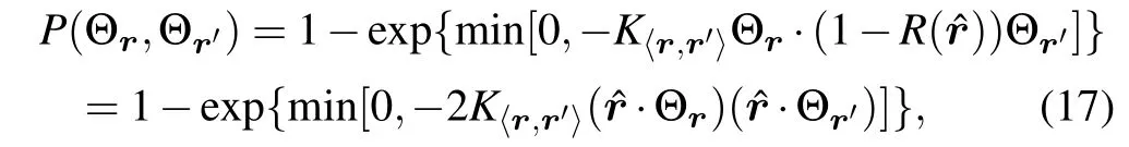
where Θrare the neighboring unit vectors as before and ˆrstands for a random unit vector pointing towards a direction within the angle of 0 to 2π. We defineR(ˆr) to be the operation of mirror symmetry along the mirror direction normal to ˆr. In one Monte Carlo update, we randomly choose one site and one vector ˆrand grow cluster in both spatial and temporal bonds, then reorient all theθrin the cluster with respect to the mirror direction normal to ˆr. The sketch map of detailed update process is shown in Appendix B.As will be shown in Subsection 4.2,the cluster update has much smaller autocorrelation time than the local and over-relaxation update schemes.

3.4. Hybrid Monte Carlo

Hybrid Monte Carlo[39,40]is widely used in high-energy physics to simulate the equilibrium distribution of manyparticle system. Its original form is the real time-evolution of classical system for classical Hamiltonian. It has also been used in the condensed matter system to carry on molecular dynamics simulation.[41]In quantum Monte Carlo, the timeevolution can generate canonical distribution and offers a way to produce the sample space of the Markov chain. There are attempts to implement it to simulate correlated electron systems,for example in a Hubbard model setting.[42,43]

Here we discuss the basic steps of HM scheme,and focus on its quantum rotor model implementation.

First, we add one auxiliary parameterprto every site in the configuration space and extend the partition function in Eq.(15)to

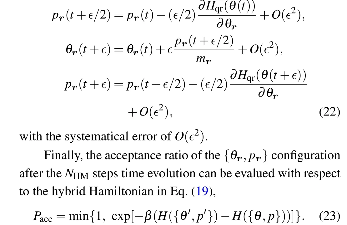
If we conductNHMtimes of the evolution,i.e.,t+NHM∊,the trajectory in the phase space will move a long distance.Such substantial update of the configuration{θr,pr}can be viewed as effectively global update, which could in principle reduce the autocorrelation time at the QCP.One point we need to pay attention to is that the detailed balance condition requests the evolution in configuration space to respect the timereversal symmetry and actually the Euler method does not satisfy this condition. So in the real simulation we use leapfrog method of Hamiltonian dynamics,

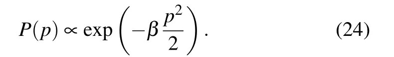
Overall, the{p}is an auxiliary degree of freedom to help to generate uncorrelated configuration in{θ}with high acceptance ratio. So after the acceptance of the update, one can easily regenerate a new{p}configuration and start the next step of the time evolution of the hybrid Hamiltonian,and can evaluate the acceptance of such step once theNHMsteps’time evolution is complete. This process is therefore the Markov chain for the hybrid Monte Carlo. To satisfy the detailed balance condition,eachpshould be generated as

We summarize the steps of HM with the pseudo-code in Table 1.

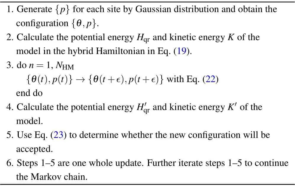
Table 1. Pseudo-code of HM algorithm.

Although HM provides an effective non-local update scheme of the original configuration space{θr}, as will be shown in Subsection 4.2, it still suffers from critical slowing down at the (2+1)dXYcritical point. And to finally overcome it, we will discuss a better Monte Carlo update scheme for the quantum rotor model: the Hybrid + Fourier acceleration method.

3.5. Hybrid+Fourier acceleration

Hybrid Monte Carlo+Fourier acceleration is designed to conquer the critical slowing down in the HM scheme. It was firstly proposed to be combined with another molecular dynamic method-Langevin equation and here we use it in the HM.[32,36]

The analysis of FA[44]reveals that the critical slowing down comes from the fact that in the internal dynamics of Monte Carlo,i.e.,at the critical point,long(short)wave length mode takes longer (shorter) time to evolve. And typical update schemes do not respect such fact and use the same time step to evolve both modes,which are consequently ended with long autocorrelation time of the Monte Carlo dynamics. To avoid this problem,one can add different footsteps to different modes to make them evolve at the same speeds,i.e.,evolve according to the internal dispersion relation of the Hamiltonian.In this way, the autocorrelation time at the critical point can be reduced,as we are now updating the configuration with the intrinsic dynamics of the Hamiltonian.

In the leapfrog process in HM scheme in Eq. (22), we take∊as the step size independent on the modes and from the discussion above,it is clear that to reduce the autocorrelation time,the proper coefficients shall depend on the evolution speed of each mode determined by the force. We can write the evolution speed for every site as

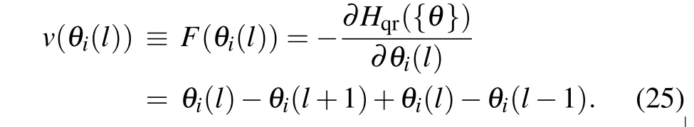
We then perform discrete Fourier transformation(DFT)along the 1D temporal chain and obtain the footstep forp-evolution,

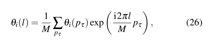
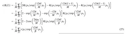
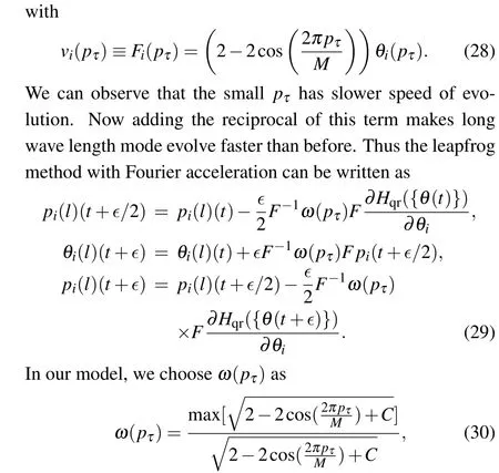
wherepτ=0,1,2,...,M-1 and Eq.(25)then becomes method is actually more versatile in terms of implementation for complicated Hamiltonians. In the Hamiltonian mechanics of Eq.(29), we actually do not worry too much about the exact form of the Hamiltonian since the updates only depend on its intrinsic dynamics. In fact,few recent examples implementing the FA scheme in the electron-phonon type of problems in 2d and 3d Holstein models where the fermions and bosons(phonons)are strongly coupled, even with long-range interactions,[44,45]have been successfully shown to reveal the interesting phenomena such as charge-density-wave transition and superconductivity.

This completes our discussion of the five different Monte Carlo update algorithms to solve the quantum rotor model and now we are ready to demonstrate our simulation results and check the different performance among the update schemes.

where the numerator is approximately equal to 2, andCis a small non-zero constant and for eachLwe choose the optimal value for it such that the autocorrelation time is the shortest and at the same it is still finite to avoidω(pτ)becoming zero.

As will be shown in Subsection 4.2,the FA scheme could greatly cure the critical slowing down in the bare HM scheme,we have succeeded in doing so by applying the Fourier acceleration along the most important direction that dominates the critical fluctuations-the imaginary time direction. The DFT is thus performed along the imaginary time direction.[44]In practice,this means we need to perform DFTL×Ltimes for every sweep.

Before the end of this algorithm section, one more point we would like to emphasize is that, although the HM plus FA scheme looks a bit more complicated than the LM, OR and WC schemes, it actually enjoys a big advantage that this

4. Results

In this section, we first use the Monte Carlo method to pin down the precise position of the (2+1)d O(2) QCP via finite size scaling analysis, then compare the performance of different update schemes at the QCP.

4.1. The(2+1)d XY quantum phase transition

We first identify the position of the quantum critical point of the quantum rotor model in Eqs.(2),(12)and(15).It can be determined by the finite size scaling analysis of the spin stiffness(in the spin language)or superfluid density(in the boson language),as

whereHα=tΔτ∑i,lcos(θi(l)-θi+α(l))is the kinetic energy of the nearest neighbor bond of both spatial directions, andIα=tΔτ∑i,lsin(θi(l)-θi+α(l))is the derivative ofHα. According to the(2+1)dXYtransition,ρswill follow the finitesize scaling function

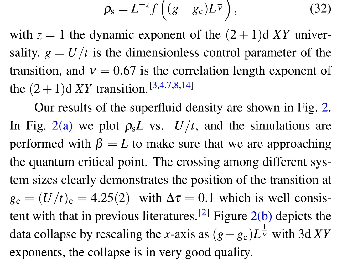
Fig.2. (a)Finite size scaling of the superfluid density according to Eq.(32),the crossing point determines the (2+1)d XY quantum critical point at gc =(U/t)c =4.25(2). (b) Data collapse of the above data with gc, z=1 and ν =0.6723.

4.2. Autocorrelation time analysis

With thegcdetermined, we can now explore the performance of various update schemes in the vicinity of the critical point. We first analyze the autocorrelation time of the static uniform magnetizationMat the QCP,

whereθris an unit vector with the phase between 0 to 2π.The summation is performed over the space-time volume, therefore theMis the static uniform magnetization of the O(2)order parameter(see Fig.1 for schematics). We measure the magnetization right at the QCPg=gc,and obtain its autocorrelation timeτfrom fitting the exponential decay of the autocorrelation function ofAM(t)as

wheretis the time in units of one Monte Carlo sweep, although the definition of one sweep can be slightly different among the update schemes, basically it corresponds to one complete update of the space-time lattice. The results are shown in Fig. 3. To obtain these smooth autocorrelation functions, we use 106Monte Carlo measurements in a single Markov chain to calculate theAM(t). From Fig.3(a), the exponential decays of the autocorrelation functions forL=8 andβ=Lat the QCP are clearly visible. Then one reads the autocorrelation time from such results for differentL.These results show that LM,OR and HM schemes are all suffering from the critical slowing down and the autocorrelation time increases drastically with the system sizeL. On the other hand, WC and FA have very small autocorrelation time and are for sure the suitable methods to apply here. To quantify the difference in the autocorrelation time, we take the log-log plot in Fig.3(b),and expect a power-law relation of the form

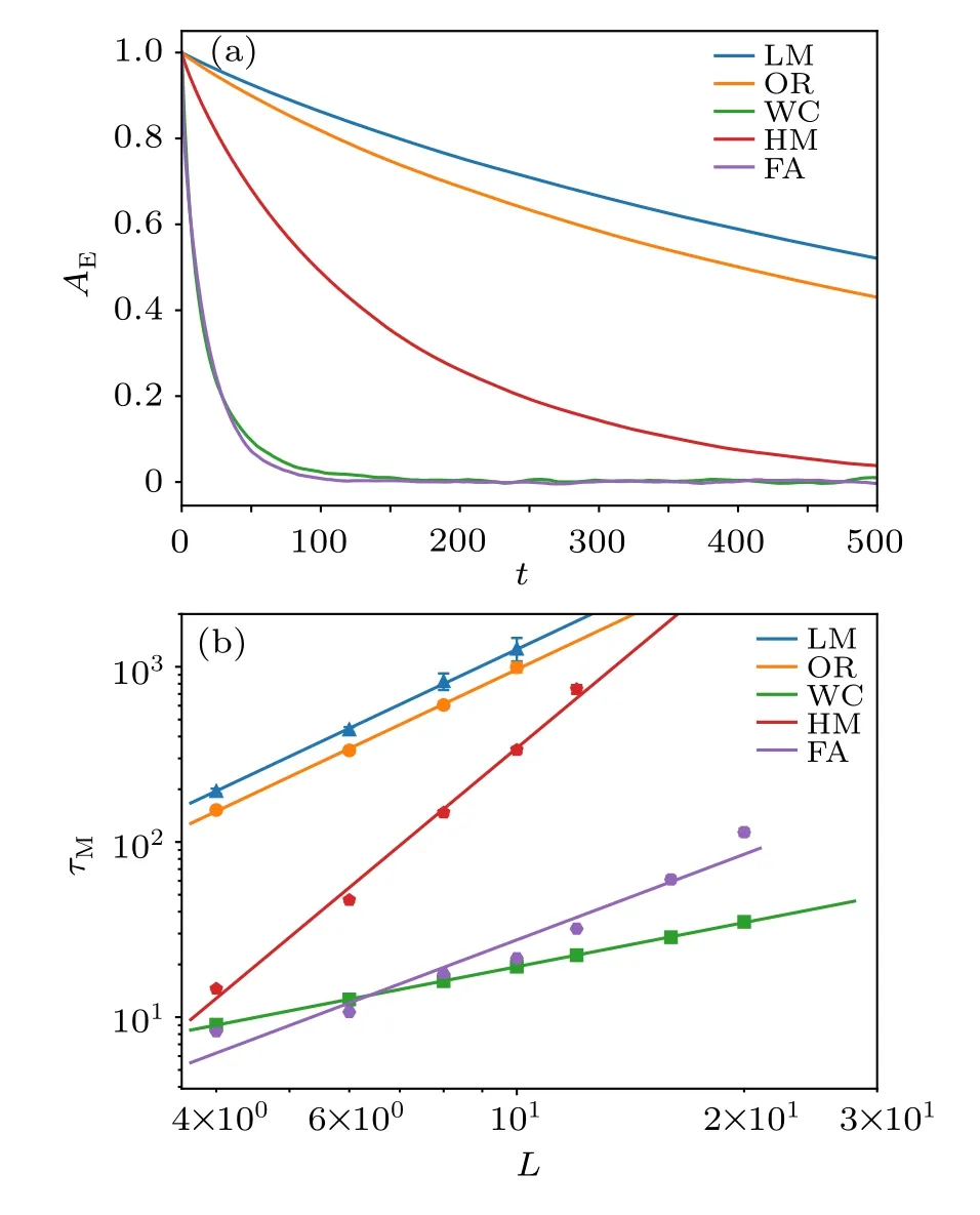
Fig.3. (a)Autocorrelation function of static uniform magnetization AM(t)in Eq.(34)at the quantum rotor QCP for LM,OR,WC,HM and FA update schemes with system size L=8 and the Monte Carlo time t is averaged over one million consecutive measurements from a single Markov chain. One can see that for LM, OR and HM, the autocorrelation time is very long,more than 500 Monte Carlo sweeps. While for WC and FA,the autocorrelation time decreases a lot. (b)Log-log plot of the autocorrelation time τM vs.L for magnetization at the quantum rotor QCP for LM, OR, WC, HM and FA update schemes. We fit the data with power-law as in Eq.(35)to obtain the corresponding Monte Carlo dynamic exponent z. As for the FA scheme,we choose C in Eq.(30)to be 0.1 for L=4,6,0.01 for L=8,10,and 0.005 for L=12,16,20,to obtain the optimal value of τM.

wherezthe dynamical exponent of the Monte Carlo update scheme, and for the 2d Ising model at its critical point, it is known that thez=2.2 for the local update andz=0.2 for the Swendsen-Wang cluster update.[18]From Fig. 3(b) one can readz=2.05(16)for LM,z=2.05(8)for OR,andz=3.60(5)for HM,and as for the other two update schemes,shorter autocorrelation times are observed,for example,z=0.84(2)for WC andz=1.62(30) for FA. So these results reveal that at the QCP of(2+1)d quantum rotor model,the critical slowing down is mostly suppressed in WC and FA schemes.

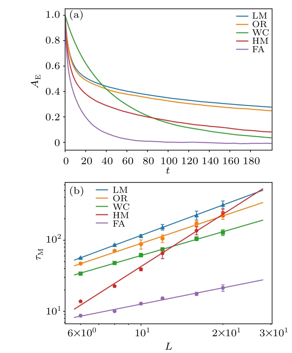
Fig. 4. (a) Autocorrelation function of energy AE(t) at the quantum rotor QCP for LM,OR,WC,HM and FA update schemes with system size L=8 and the Monte Carlo time t is averaged over one million consecutive measurements from a single Markov chain.One can see that for LM,OR and HM,the autocorrelation time is very long,more than 200 Monte Carlo sweeps. While for WC and FA, the autocorrelation time decreases a lot. (b) Log-log plot of the autocorrelation time τE for energy at the quantum rotor QCP for LM,OR,WC,HM and FA update schemes. Again we fit the data with power-law as in Eq.(35),to obtain the corresponding Monte Carlo dynamic exponent z.As for the FA scheme,we choose C in Eq.(30)to be 0.1 for L=6,8,10,12,and 0.005 for L=16,20,to obtain the optimal value of τE.

The same analysis can be performed for the autocorrelation time of energy at the QCP, and the results are shown in Fig. 4, one can readz=1.40(11) for LM,z=1.28(8) for OR, andz=2.43(12) for HM. As for the other two update schemes,shorter autocorrelation times are observed,for example,z=1.11(6)for WC,and most importantly,z=0.76(8)for FA with the smallest autocorrelation time of all sizes. It illustrates that the autocorrelation time for energy is different from that for the magnetization - it is actually normal since different physical observables can have different autocorrelation time-these results nevertheless reveal the consistent picture that at the QCP of(2+1)d quantum rotor model, the critical slowing down is mostly suppressed in WC and FA schemes.

4.3. CPU time analysis

Besides the autocorrelation time and its scaling with system size at the QCP,we also test the effective calculation time of each Monte Carlo scheme.

For example,for the magnetization atL=8,β=Lat the QCP, we compute the real CPU time and the obtained errorbars among different schemes. Here,we use method of rebinning to estimate the errorbar of data for each update scheme and the time it takes to reach that. As shown in Fig. 5, with fixed sample number of magnetization, we group the data of everynconsecutive measurements into one bin,then calculate errorbar of sample mean among these bins. As the bin sizenbecomes large,the correlation of sample mean among the bins becomes small,and an plateau of the errorbar will be reached once the data among different bins are indeed statistically independent. Among different schemes, it is clear that for WC and FA schemes, not only the plateaus in errorbar are reach at the earliest,aroundn～100 of the bin size,but also the intrinsic errorbars obtained in this way are actually the smallest among the five update schemes. These results imply that the WC and FA schemes will be able to acquire the best quality data with the smallest intrinsic errorbars of the magnetization at the QCP with the shortest CPU time. All the other schemes,LM,OR and HM,will take much longer time for the intrinsic plateaus of their errorbars to be reached and hence will take longer CPU time.

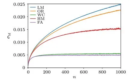
Fig.5. The rebinning of the static uniform magnetization of different algorithms as a function of bin size n. We choose the L=8 and β =8 system at the QCP, and rebin the consecutive measurements to obtain the intrinsic errorbars σM of different update schemes. It is clear for WC and FA, the plateaus of errorbar are already reached when n ＜200, and for the other update schemes,it will take much longer CPU time for the intrinsic errorbar plateaus to be reached,if ever reached.

The actual CPU hour spent on achieving the errorbar of order 0.001 for the static uniform magnetization is shown in Fig.6. As explained above,it is indeed the case that the HM,LM,OR schemes need longer physical time to achieve the required level of statistical error and among these three,the FA scheme is the slowest mainly due to the leapfrog processes therein, although it shows smallerτMandτEcompared with LM and OR schemes. The FA and WC schemes,on the contrary, need very few CPU hours to achieve the required error and the WC is the best in this regard. But it should be mentioned that although the FA scheme spends longer physical time than WC mainly due to its computational complexity.It introduces more adjustable coefficients such asNHM,∊,andω(pτ),and it offers the opportunity of efficient global update even if the Hamiltonian of the problem at hand is more complicated, such as the fermion-boson coupled systems aforementioned, where usually long-range interactions are present and one can no longer construct WC type of update.

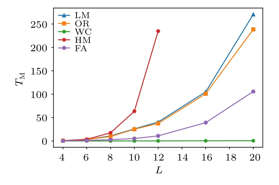
Fig.6. The CPU hour TM spent for each Monte Carlo scheme to obtain the error of 0.001 of static uniform magnetization M, as a function of system sizes L. As expected, although the HM scheme has shorter autocorrelation time compared with LM scheme,it actually spends more CPU time on obtaining the shorter autocorrelation time mainly due to the leapfrog processes therein. Whereas with FA scheme,both the autocorrelation time and the CPU hour spent are much less compared with LM, OR, HM schemes in reaching the same errorbar. The less CPU hours spent are for the WC scheme, owing to both the small autocorrelation time and less number of operations in the algorithm, thus it will be the best to calculate the bigger size quantum rotor model.

5. Discussion

In this paper, we systematically test the performance of several Monte Carlo update schemes for the (2+1)d O(2)phase transition of quantum rotor model. Our results reveal that comparing the local Metropolis, local Metropolis plus over-relaxation, Wolff-cluster, hybrid Monte Carlo, hybrid Monte Carlo with Fourier acceleration schemes,it is clear that,at the quantum critical point,the WC and FA schemes acquire the shortest autocorrelation time and cost the least amount of CPU time in achieving the smallest level of relative error.

As we have repeatedly discussed throughout the paper,although the(2+1)d quantum rotor models have been satisfactorily solved with various analytic (such as high temperature expansion,[7,8]conformal bootstrap[9])and Monte Carlo simulation schemes, it is now becoming more clear to the community that the extension of quantum rotor model to more realistic and yet challenging models, such as quantum rotor models-playing the role of ferromagnetic/antiferromagnetic critical bosons,[22,23]Z2topological order[46]and U(1)gauge field in QED3[24,25]-Yukawa-coupled to various Fermi surfaces will provide the key information upon the important and yet unsolved physical phenomena ranging from non-Fermiliquid, reconstruction of Fermi surface beyond the Luttinger theorem[47-50]and whether the monopole operator is relevant or irrelevant at QED3with matter field.[25,51]Furthermore,the bosonic fluctuation may even be applied in the momentum space,e.g.,the twisted bilayer graphene.[52]And progresses in the problem of Fermi surface Yukawa-coupled to the quantum rotor model[53,54]have been made by some of us,in which,we combine three of five update schemes discussed in the present work, and show that they together give us a general pattern in effectively sampling the O(2) bosons in the coupled systems. Novel physical phenomena including the non-Fermiliquid quantum critical metal,the deconfined critical point,[55]and the pseudogap and superconducting phases which are generated from the quantum critical bosonic fluctuations,are discovered from QMC simulations.

Moreover, although the fundamentalness of these questions go way beyond the simple(2+1)d Wilson-Fisher O(2)fixed point,but the successful solution of these questions heavily relies on the design of more efficient Monte Carlo update schemes on the quantum rotor or O(2)degree of freedoms in the (2+1)d configuration space of the aforementioned problem. In the presence of the fermion determinant, one can perform the traditional determinantal quantum Monte Carlo method with local update of the O(2) rotors for small and medium system sizes, then with the available self-learning and neural network schemes,[27-29]an effective model with non-local interactions among the rotors can be obtained which serves as the low-energy description of the fermion-boson coupled systems. Then the methods tested in this paper, in particular the hybrid Monte Carlo with Fourier acceleration scheme, can be readily employed to perform global update for such effective model,which will certainly reduce the autocorrelation time compared with the simulation of the original model and consequently reduce the actual CPU hours spent in achieving the same level of numerical accuracy of the physical observables. Recent progress in the Holstein-type problems,where fermions and phonons(bosons)are strongly coupled in 2d and 3d lattices with long-range interactions with FA scheme,has been shown to be successful in revealing various charge-density-wave and superconductivity transitions.[44,45]

Acknowledgements

We thank Ying-Jer Kao for insightful discussion and introduction to us the over-relaxation update scheme in Ref.[5].WLJ,GPP,YZL and ZYM acknowledge the supports from the Strategic Priority Research Program of the Chinese Academy of Sciences(Grant No.XDB33000000)and the RGC of Hong Kong SAR of China (Grant Nos. 17303019, 17301420, and AoE/P-701/20). We thank the Center for Quantum Simulation Sciences in the Institute of Physics,Chinese Academy of Sciences, the Computational Initiative at the Faculty of Science at the University of Hong Kong, the National Supercomputer Center in Tianjin, and the National Supercomputer Center in Guangzhou for their technical support and generous allocation of CPU time.

Appendix A:Link-current representation

where ΔEr=E＇r-ErandE＇randErrepresent the classical energy after and before the update on bond〈r,r+µ〉described by Eq. (A1). Thus the probability can be derived by normalizing the weightpr,μ=Ar,μ/Nr,whereNr=∑μ Ar,μ.Usually, we add the same integer to all bonds on the loop to satisfy the continuity equation Eq.(A2).

Moreover,transferring the lattice to its dual one can avoid the constraint, as the Monte Carlo update with constraint is usually difficult to implement. One can easily update one site instead of a loop,by writing

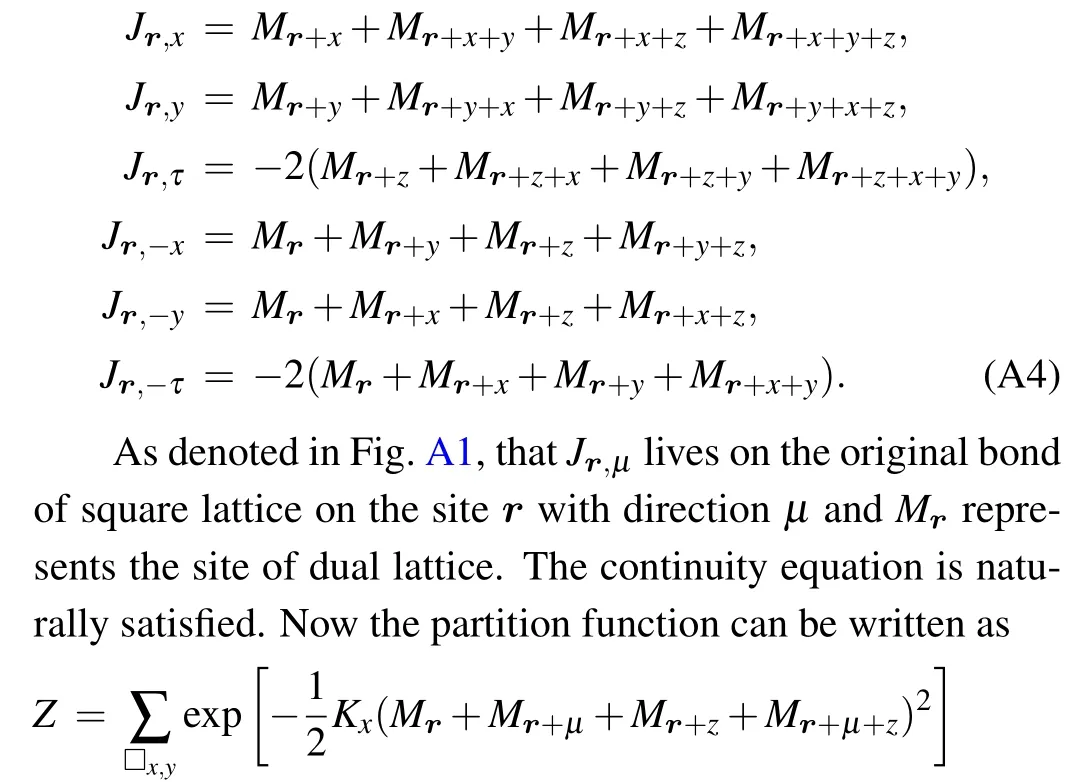
Here,µrepresentsxandydirections. The summation in the first line of Eq. (A5) runs over all the square whose normal vector is in the directions ofxandy. Similarly,the summation in the second line of Eq.(A5)runs over all the square whose normal vector is in the direction ofz. Local update can be easily used in this situation of one site by simply calculating the energy difference of the square it locates.

Fig.A1. Map from the original lattice to dual lattice according to Eq.(A4).

Appendix B:WC update scheme

Here we show the detailed update process by means of part of sites in the whole system. Four subgraphs in Fig. B1 show the vectors before update,choosing the random site and mirror denoted by ˆr,construct the cluster with probability,reorient the vectors,respectively.