Traffic flow prediction based on BILSTM model and data denoising scheme

Zhong-Yu Li(李中昱) Hong-Xia Ge(葛红霞) and Rong-Jun Cheng(程荣军)

1Faculty of Maritime and Transportation,Ningbo University,Ningbo 315211,China

2Jiangsu Provincial Collaborative Innovation Center for Modern Urban Traffic Technologies,Nanjing 210096,China

3National Traffic Management Engineering and Technology Research Center Ningbo University Subcenter,Ningbo 315211,China

Keywords: traffic flow prediction,bidirectional long short-term memory network,data denoising

1. Introduction

Traffic flow prediction is an important component of intelligent transportation system, which can reduce the number of accidents,improve traffic efficiency,and reduce traffic pollution. The traffic prediction is based on a large number of historical data to predict the future traffic flow.[1]Previous studies show that linear model, nonlinear model, and hybrid model are three typical traffic flow prediction techniques.[2]In the linear models the mathematical methods are used to complete the task of the traffic flow prediction. The autoregressive integrated moving average model (ARIMA) is the most commonly used linear model.[3]Chenet al.[4]proposed an ARIMA model. The ARIMA model was specified by different training data, which represent the different traffic states,according to the different periods in different days. The model from different periods would be used on different data when testing. This would make the model more special and more accurate. The data-driven approach using the ARIMA model in most of studies required sound database for building a model. The seasonal ARIMA method was proposed to predict the short-term traffic flow with limited data.[5,6]Although the ARIMA had good prediction accuracy,there were many nonlinear factors in traffic flow prediction. Therefore,the nonlinear models introduced relevant machine learning methods(including support vector regression(SVR),artificial neural networks(ANN),etc.)to achieve favorable traffic flow prediction performance.The SVR had strict theoretical and mathematical basis. Based on the principle of structural risk minimization,it has strong generalization capability and global optimality. It was a theory for small sample statistics.[7-10]Neural network had strong non-linear fitting capability and could learn rules from large samples. Moreet al.[11]predicted the future traffic volume through the ANN,and used the predicted results to control congestion. Kumaret al.[12]used the ANN to make short-term prediction of traffic volume by using past traffic data (taking the traffic volume, speed and density as inputs).The ANN can produce good results in this study. In order to better capture the spatiotemporal information of traffic flow,convolutional neural network has been proposed.[13-15]In order to better learn the historical information of data,recurrent neural network(RNN)was proposed to be able to transfer the output of the previous time to the next step as input, thereby improving the accuracy of prediction.[16]The RNN can handle certain short-term dependence, but it cannot handle the longterm dependence. To solve this problem,the LSTM was proposed.The LSTM introduced cell state,and the input gate,forgetting gate and output gate were used to maintain and control the information,which can learn long-term information.[17]It is noted that the nonlinear models have achieved great success in dealing with many traffic flow prediction tasks. However,the uncertainty of traffic flow data might have a negative effect on the nonlinear prediction model, which would reduce the performance of the model. The hybrid models were proposed to overcome the disadvantages.[18,19]For example,Tanget al.[20]combined fuzzy c-means and genetic algorithm to predict missing traffic volume data. Zhenget al.[21]used a hybrid model based on a convolutional neural network(CNN)and the LSTM.The experimental results show that the prediction accuracy of the hybrid model is higher than that of the single model.

Traffic flow data can be obtained by many technical means, such as remote microwave, loop deductive detectors,global positioning system(GPS).[22]Historical data with high fidelity play a critical role in predicting results, but raw data always contain noise. Therefore, one introduced many noise reduction methods,[23]such as the wavelet Kalman filter model[24,25]and wavelet transform.[26,27]Yanget al.[28]selected the appropriate wavelet basis to decompose and reconstruct the traffic flow data. The results showed that prediction effect is better than the results predicted just by neural network in prediction precision and network convergence. Because the wavelet transform needed to select the appropriate wavelet base, sometimes it is difficult to find the appropriate wavelet base. One proposed the EMD,which is an adaptive decomposition method based on the original data.[29]The EMD extracts the intrinsic mode function(IMF)sets from the input data samples, which can be separated into high-frequency (HF) part and low-frequency (LF) part. The EMD is affected by mode mixing,so the EEMD was proposed.[30,31]Chenet al.[32]proposed an integrated framework based on the integrated EEMD and the ANN can predict the traffic flow at different time intervals ahead. The experimental results show that the noise reduction algorithm greatly improves the accuracy of traffic flow prediction.

The above method combines a certain noise reduction method with the prediction method to achieve better prediction accuracy, but does not use the same set of data to verify the performance of different noise reduction algorithms. The present study intends to combine data denoising algorithms with deep learning model to predict the traffic flow and compare among prediction accuracies of various methods. The contributions of this paper are as follows:

(i)We use denoising algorithms to process the raw data,which include WL,EMD,and EEMD,and compare the capabilities of these algorithms to suppress the outliers.

(ii) We build a BILSTM prediction model to predict the data already processed.

(iii)We consider the predicted effects of the model under different road scenarios(i.e.,mainline,on ramp,off ramp)and on different time scales(i.e.,5 min,10 min,and 15 min).

The rest of this paper is organized as follows. In Section 2,the denoising methods and BILSTM are introduced. In Section 3,the source of data,the model structure,and prediction results are presented. In Sections 4 some conclusions are drawn from the present study.

2. Method

The methods to be used in this article are data denoising and deep learning neural networks to improve prediction accuracy. The frame of this model is shown in Fig.1.

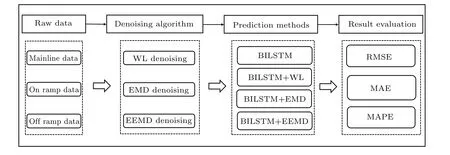
Fig.1. Framework of prediction model.

2.1. Denoising methods

2.1.1. Wavelet

Wavelet is used to eliminate noise interference in traffic flow data.[33]The purpose of building a noise reduction model is to reduce the influence of interference factors,such as gaussian noise,on the prediction accuracy of the model in a complex,nonlinear traffic data set. One-dimensional noise model can be expressed as

whereFtis the raw signal with noise;ytis the signal without noise;εtis Gaussian noise;nis the signal length. The principle of wavelet denoising is to suppress theεtpart ofFtand restore theytpart ofFt. Wavelet denoising model preserves the original signal characteristics after denoising. The flow chart of wavelet is shown in Fig.2. The wavelet algorithm is implemented in three steps.

Step 1 Decomposition

Choose a wavelet and determine the layerNfor a wavelet decomposition,then compute theN-layer wavelet decomposition for the signal.

Step 2 Setting a threshold for high-frequency coefficients

For the high-frequency factor of each layer from layer 1 to layerN,a threshold is selected for thresholding.

For most of signals,the low-frequency component is very important,and it usually contains the characteristics of the signal, while the high-frequency component contains the details or differences of the signal. The low-frequency information can approximately describe the change trend of the original signal, while high-frequency information represents the detailed information of the signal. Therefore,the original signal can produce two signals (high- and low-frequencies) through two mutual filters.

Step 3 Data reconstruction

According to the approximate coefficients and the modified wavelet coefficients,the inverse wavelet transform is used to reconstruct the traffic data after denoising.

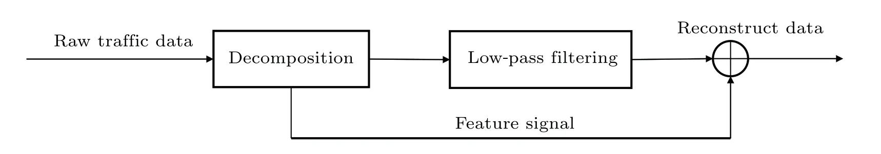
Fig.2. Flowchart of wavelet.

2.1.2. The empirical mode decomposition (EMD)

In this paper, we use the EMD, which was first introduced by Huanget al.[34]Different applications in medical signal analysis have shown the effectiveness of this method.The principle is to adaptively decompose the given signal into frequency components,which called intrinsic mode functions(IMF).These components are obtained from the signal by an algorithm. The algorithm extracts the highest frequency oscillation of each mode from the original signal. The more detailed explanations to the EMD model are described as follows.

(i)Decompose raw traffic flow dataR(t)into IMFs. Find out potential extreme points fromR(t) data series, then employ the cubic spline interpolation method to connect the maximum and minimum points to form the upper envelopeU(t)and lower envelopeL(t).

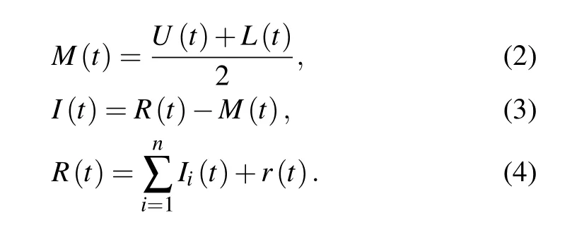
(ii) Calculate the mean of the upper envelopeU(t) and lower envelopeL(t) to obtain the mean envelopeM(t) (see Eq.(2)).

(iii) Calculate the difference betweenR(t) andM(t) to obtainI(t)(see Eq.(3)). IfI(t)satisfies the IMF’s conditions,I(t) is one of the IMFs, otherwise the above three sub-steps need repeating untilI(t) satisfies IMF’s condition. The following IMF’s conditions are satisfied:i)the number difference between extrema and the zero-crossing points is not larger than one;ii)at any point in the IMF,the mean value of the envelope defined by the local maximum and the mean value of the envelope defined by the local minimum should be equal to zero.

(iv)Obtain the residual partr(t)by calculating the difference betweenR(t)andI(t),repeat the above three sub-steps to obtain new IMFs until the residual data distribution is monotonic or has one extreme point. Finally,R(t) is decomposed into a series of IMFs and a residual partr(t)as shown by the following equations:

2.1.3. The ensemble empirical mode decomposition(EEMD)

For some data with too few extreme points, EMD fails to work, so the EEMD method is proposed. The white noise is added into the EEMD to make the data meet the requirements for the EMD. Owing to the zero mean white noise,the zero mean white noise will cancel each other after many times of average calculation, so the calculation result of integrated mean can be directly regarded as the final result. The EEMD can effectively suppress the mode aliasing of EMD.The EEMD algorithm steps are as follows.

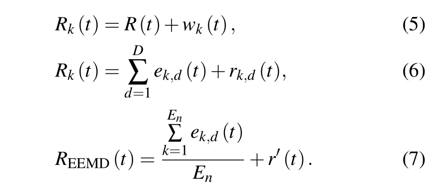
Step 1 The white noisewk(t) of normal distribution is added into the raw traffic dataR(t)(the noise-aided traffic flow data are denoted asRk(t))(see Eq.(5)).

Step 2 TheRk(t) are decomposed into IMFs and residual components. The data decomposition program will be executed in thek-th round until the conditionk ＞Enis met(Enis the ensemble number). TheRk(t)data can be decomposed into IMFsek,d(t)and corresponding residual partrk,d(t)(see Eq.(6)).

Step 3 Repeat steps 1 and 2,add a new normal distribution white noise sequence each time.

Step 4 Select the noise-free IMFs and residuals to reconstruct the EEMD smoothed traffic flow dataR(t)EEMDwhich are given below:

2.2. Deep learning

2.2.1. Long short-term memory (LSTM) network

The LSTM is an improved neural network based on recurrent neural network (RNN). The LSTM was proposed by Hochreiter and Schmidhuber in 1997.[35]In the RNN the output of the previous moment is taken as the input of the next moment,and the RNN is often used to predict the data of time series. However,the RNN tends to disappear and explode gradients when dealing with long sequences,leading the model to be nonconvergent.To solve this problem,the input gate,forget gate, output gate, and memory cell (C(t)) are added into the LSTM.The LSTM structure is shown in Fig.3.

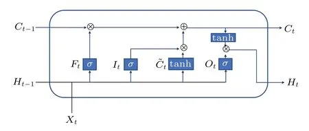
Fig.3. LSTM structure.

The three gates are connected by the Sigmoid activation function. The Sigmoid activation function is a hyperbolic tangent function, and the value field is controlled in an interval of[0,1]. Candidate memory cells(˜Ct)are connected by tanh activation function,and the range was controlled in an interval of[-1,1]. The calculation steps of the model are as follows:

whereI(t),F(t),O(t),and ˜C(t)represent the input gate,forget gate, output gate, candidate memory cells, respectively;Wxi,Whi,Wx f,Whf,Wxo,Who,Wxc,andWhcare the weight matrices.bi,bf,bo, andbcare bias vectors.σis a Sigmoid activation function.

Memory cell (Ct) is obtained fromCtand ˜Ct. Then we acquireHtby combining ˜Ctwith the tanh activation function as follows:

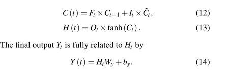
2.2.2. Bi-directional long short-term memory network(BILSTM)

The Long short-term memory is a forward training model,which can only capture the long-term characteristics of forward historical traffic flow data. However,the traffic flow data not only depend on past information, but also correlates with future road conditions. The BILSTM is an optimized LSTM model,which combines forward LSTM and reverse LSTM to obtain the information. Therefore, the BILSTM can process and integrate data forward and backward,which can make the prediction more accurate. The BILSTM structure is illustrated in Fig.4. The forward layer and backward layer are connected to the output layer,which contains six shared weights.

Fig.4. Structure of BILSTM.

In the forward layer,the forward calculation is performed from timelto timet, and the output of each forward hidden layer is obtained and saved. In the backward layer, the output of the backward hidden layer at each time is obtained and saved by backward calculation from timetto timel. Finally,the final output is obtained by combining the output results of forward layer and backward layer at each time,the calculation steps of the model are as follows:

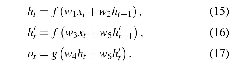
In Fig.4,xtrepresents the input of LSTM,Ofdenotes the output of forward LSTM,andObrefers to the output of reverse LSTM.

3. Experiments

3.1. Data source

The traffic flow data in this paper are obtained from the performance measurement system (PeMS). The PeMS is an intelligent traffic management tool. It collects and stores realtime traffic data from sensors and provides online use. The PeMS data collection covers major metropolitan areas in California. We collected the traffic flow data from three detectors installed in Interstate 15 (I15) freeway segment located in San Diego, California (see in Fig. 5). The three detectors are located in mainline(denoted as detector A),on-ramp(represented as detector B), and off-ramp (marked as detector C)(see in Fig. 6) respectively. Owing to the different road conditions of these three sections, the predictions of these three sections can better illustrate the effectiveness of the model.We selected 2880 data in total from weekdays 1 March 2021 through 12 March 2021, and took the flow every 5 min. The details of the road sections are shown in Table 1.

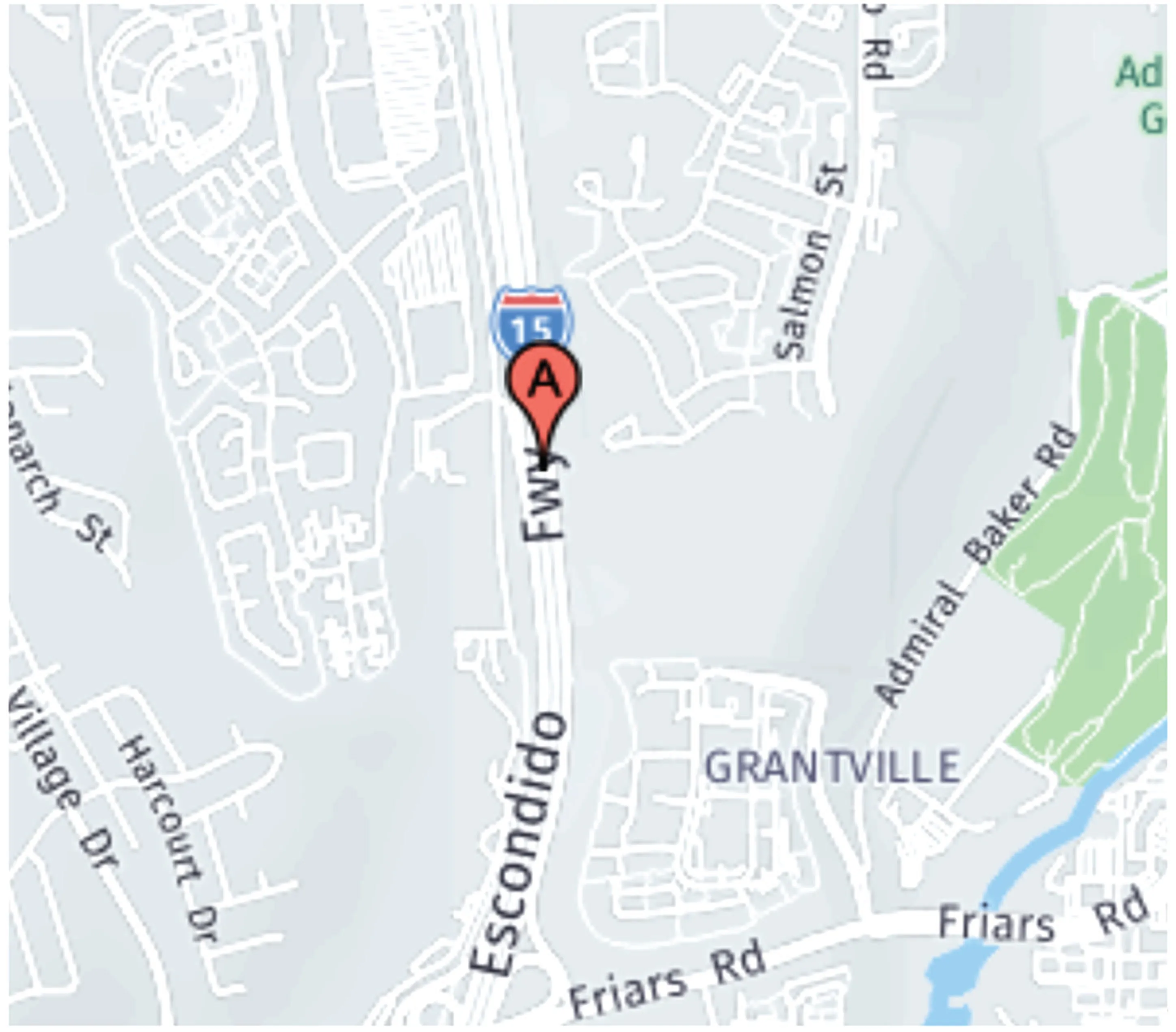
Fig.5. Interstate 15(I15)freeway segment.

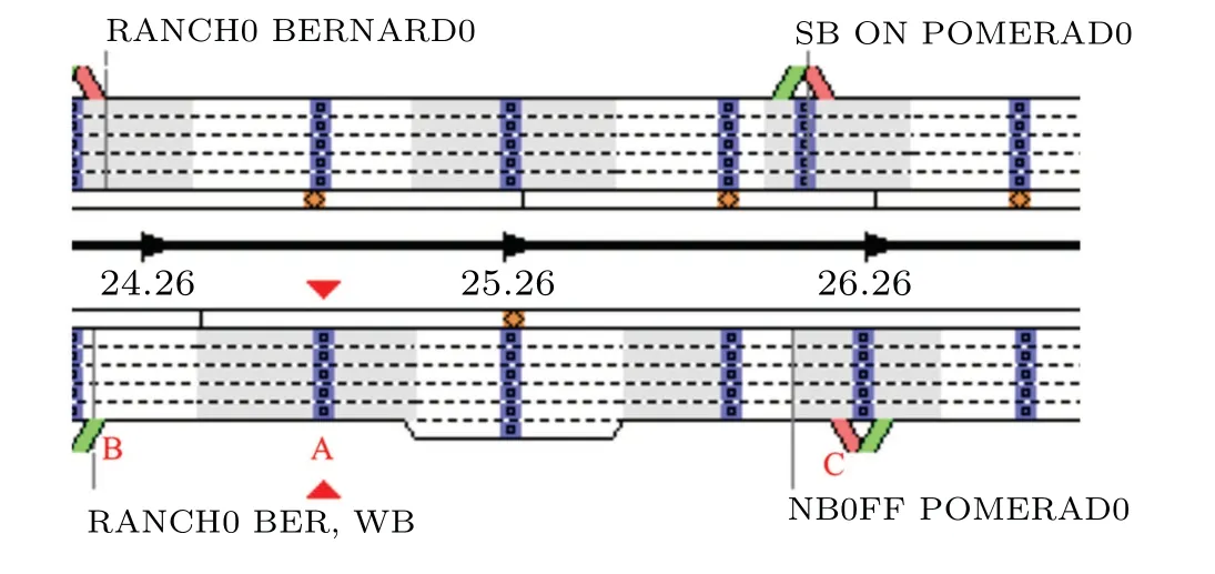
Fig.6. Three detectors.

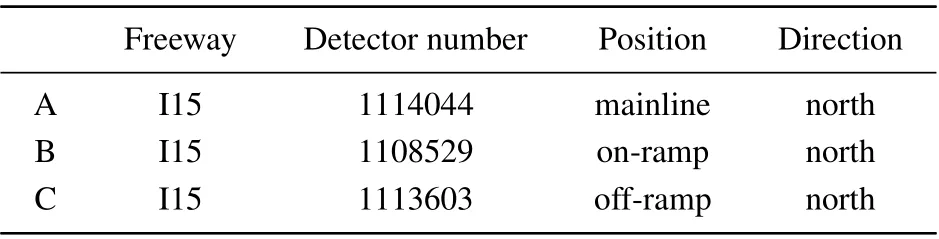
Table 1. Details of road sections.

3.2. Experiment setups

Firstly, the data are subjected to noise reduction. The wavelet denoising is a very common denoising method. It has many wavelet bases. Four commonly used wavelet bases are selected in this paper: WL (db4), WL (coif), WL (sym), and WL (haar). When using wavelet denoising, we set the number of decomposition layers to be 3 and the wavelet bases are assumed to be db4,coif2,haar,and sym2 respectively. In using EMD, we set the number of IMF decompositions to be 5, and the interpolation used is pchip (piecewise cubic Hermite interpolating polynomial method). In using EEMD,there are two parameters (the standard deviation ratio between the added Gaussian white noise and the amplitude of the input signal,An, and the ensemble number,En)need to be set. We setAn=0.2 andEn=1000. We use Adam gradient descent algorithm in BILSTM.The data are used four times to make a prediction once. We divide 70%of the raw traffic data as the training dataset and 30%as the test dataset,use Adam gradient descent algorithm,then train 500 times to obtain the prediction results.

3.3. Evaluation of predictive performance of model

The root mean square error (RMSE), the mean absolute error(MAE),and the mean absolute percentage error(MAPE)are used to evaluate the prediction performance of the model.The RMSE,MAE,and MAPE are calculated as follows:

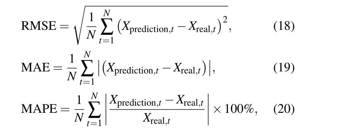
whereXprediction,tis the prediction results,Xreal,tis the raw traffic data,andNis the data-sampling number.

3.4. Results

3.4.1. Traffic flow data denoising for detector A

We employ the wavelet model, EMD, EEMD to remove outliers from original data. In order to see clearly, the noise reduction results of the first 1000 data are shown in Fig. 7.The reliable data are provided for subsequent prediction,blue lines on the plots represent denoised data, and red lines refer to the raw data. The data of a day is 288,and we can see that these data are periodic. It can be observed that the traffic flow in a day can be divided into peak period and flat peak period.The fluctuation of the data in the peak period is significantly higher than that in the flat peak period. This is because the road occupancy rate is high in the peak period and the driving behaviors of drivers will have a great influence on the road conditions, so the noise of the traffic flow in the peak period will be much higher than that in the flat peak period. It can be seen that the noise interference in the flat hump period is less,and the noise reduction results are almost consistent with the raw data. It can be seen that the curve of data after noise reduction are significantly smoothened than that of the original data,which smoothens the fluctuations from the original data.As shown in Fig.7, WL(coif2)denoised data (see Fig. 7(a))and WL(db4)denoised data(see Fig.7(b))are better than WL(haar)denoised data(see Fig.7(c))and WL(sym2)denoised data(see Fig.7(d))in data denoising. The curve of EEMD denoised data is smoother than that of the EMD denoised data.

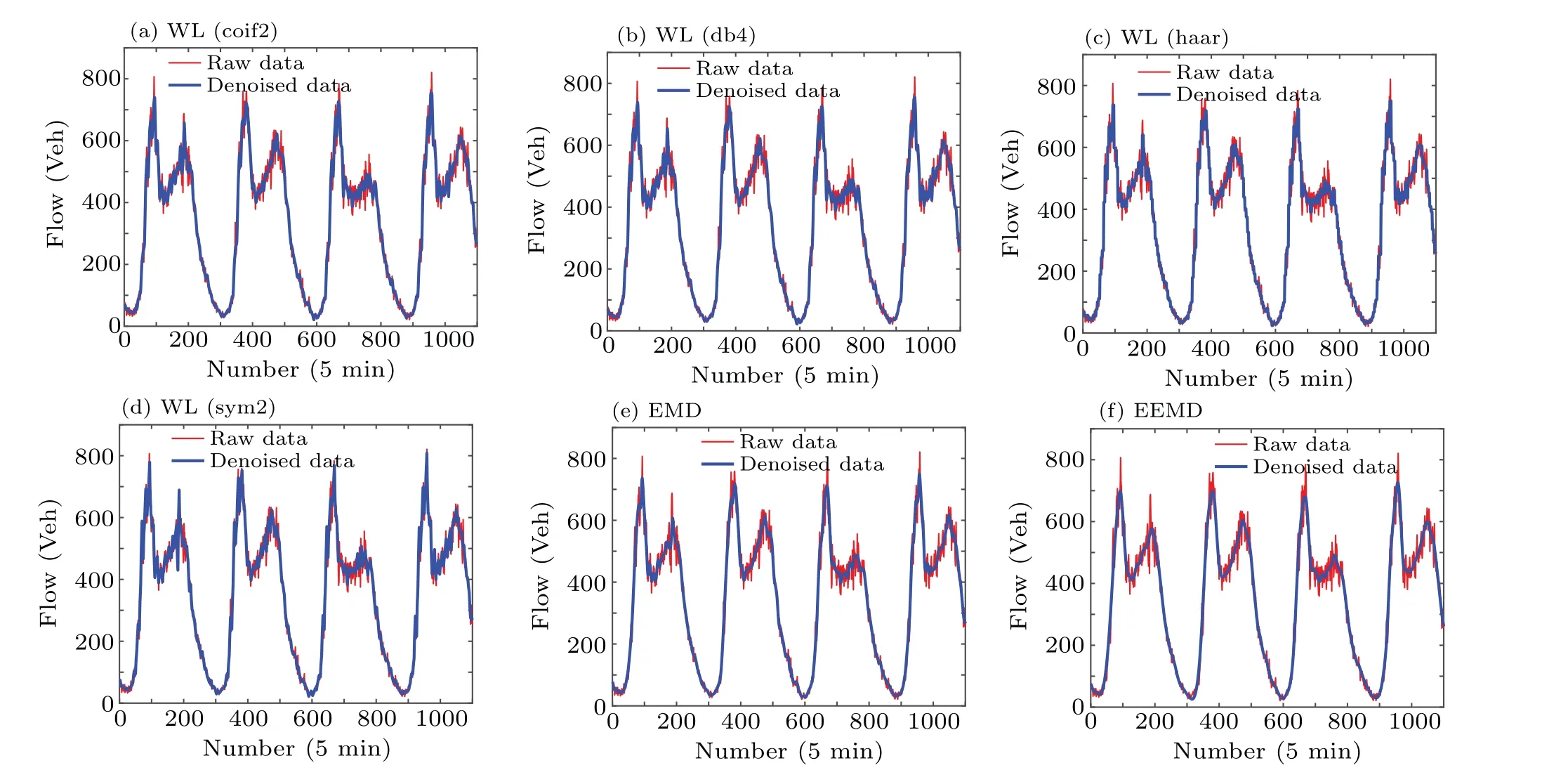
Fig.7. Denoising results for detector A.

3.4.2. Predictions for detector A

Now, we come to acquire the smooth data and use the BILSTM model to make predictions for detector A.The traffic flow prediction schemes are denoted as follows: BILSTM,BILSTM+WL (coif2), BILSTM+WL (db4), BILSTM+WL(haar), BILSTM+WL (sym2), BILSTM+EMD, and BILSTM+EEMD. The predicted results are shown in Fig. 8.The black line represents the raw data and the red line denotes the predicted data. The results of RMSE, MAE, and MAPE are shown in Table 2.The RMSE,MAE,and MAPE measured directly from BILSTM are 30.68, 22.70, 8.76%, respectively(see Table 2). The predicted RMSE decreases by 20% after noise reduction. It can be seen that the data after noise reduction can be predicted to better learn the change trend of traffic flow and improve the predict accuracy.

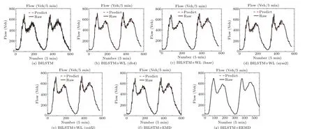
Fig.8. Results of prediction(detector A).

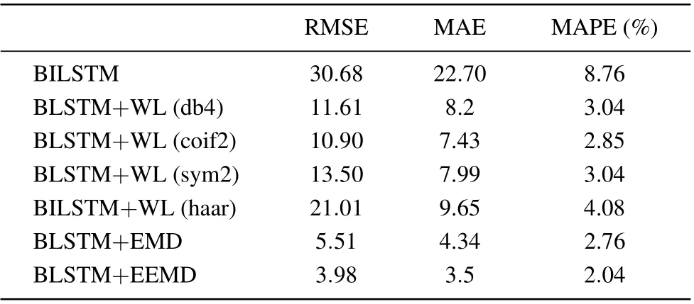
Table 2. Results of different prediction models for detector A.

Furthermore, we can see that the EEMD has the best effect. The RMSE,MAE,and MAPE of BILSTM+EEMD(see Table 2) are 3.98, 3.5, and 2.04% respectively. The performances of EEMD and EMD combined with the BILSTM are better than that of wavelet combined with the BILSTM, indicating the excellent performance of EMD with respect to EEMD in eliminating data anomalies.

3.4.3. Traffic flow data prediction and denoising for ramp detectors B, C

To further validate the performance of the model,we will take the data from ramp detectors(detector B,detector C)for prediction.

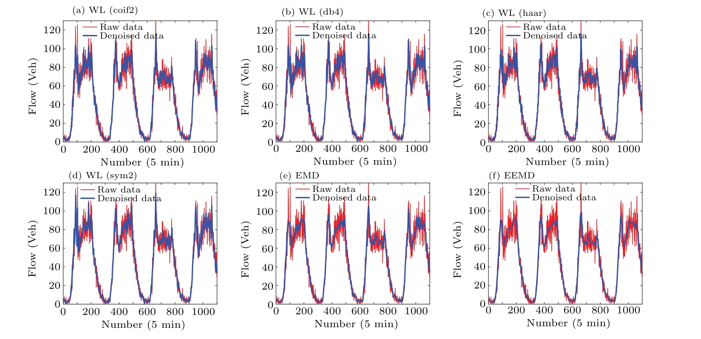
Fig.9. Denoising results for detector B.

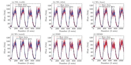
Fig.10. Denoising results for detector C.

Since the road situation of the ramp is different from that of the main line, we verify the predictive capability of the model in different road situations. The data denoising results for the two detectors are shown in Figs.9 and 10,respectively.The noise reduction procedure effectively suppresses outliers from the raw traffic data.

The prediction performance for detectors B and C are shown in Tables 3 and 4. The RMSE, MAE, and MAPE for BILSTM of off ramp (see in Table 3) are 9.43, 6.76,and 24.98%, respectively. The RMSE, MAE and MAPE for BILSTM+WL(coif2)of off ramp(see Table 3)are 1.96,1.39,and 5.50%,respectively. The accuracy of noise reduction prediction from the wavelet method is improved by about 50%.Table 3 indicates that the BILSTM+EMD scheme is better than BILSTM combined with wavelet. In Table 4,we observe that the prediction distributions are the same as in Table 2.Moreover,the prediction accuracy of BILSTM+EEMD model for detector B and detector C are better than those of other hybrid models.The RMSE,MAE,and MAPE are 0.74,0.62,and 1.75 for the traffic flow data collected from detector B,and the statistical values are 0.68, 0.49, and 2.42 collected from detector C.Through the above analysis,it can be concluded that the BILSTM+EEMD model shows the predicted performance consistent with the traffic flow data collected from mainline,on-ramp, and off-ramp areas. This means that the hybrid model is suitable for different road conditions.

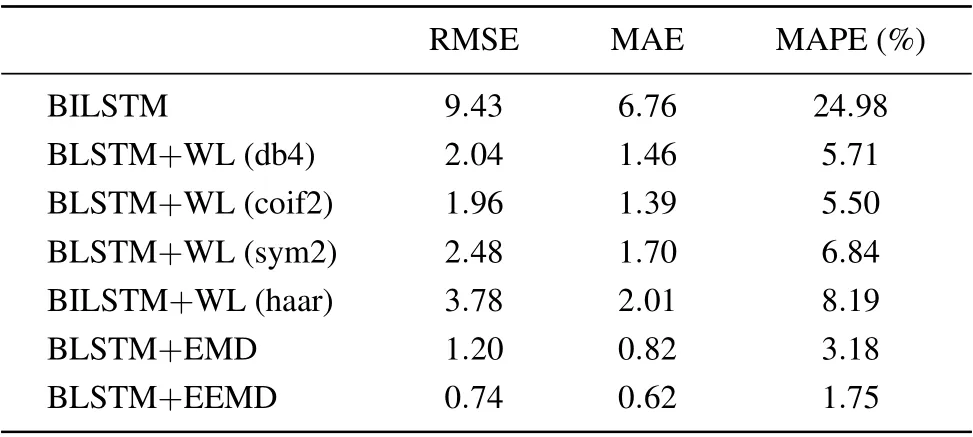
Table 3. Results of different prediction models for detector B.

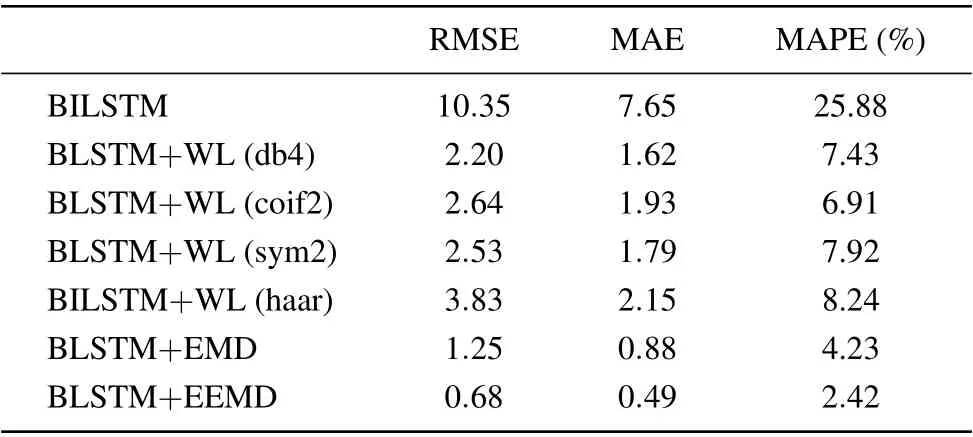
Table 4. Results of different prediction models for detector C.

3.4.4. Comparison among traffic flow data prediction for detectors A, B, and C

In order to study the influence of noise on different roads,we will add the prediction effect of noise reduction under three road conditions: mainline, on-ramp, and off-ramp. The predicted results are shown in Tables 2-4, so we select the results of EEMD for comparisons. The comparison is shown in Table 5. It can be seen that the accuracy of the model is greatly improved after noise reduction. The prediction results of off ramp and on ramp are similar. After noise reduction,the MAPE of the ramp decreases greatly in comparison with that of the mainline. It can be seen that the noise has a greater influence on the ramp. According to the analysis of traffic flow state in reality,the ramp is only a one-way line,and there are more uncertain factors in the driving of vehicles. The noise in the data is not only increased with the increase of traffic flow,but also related to many factors, such as the weather and the working state of loop detector. The traffic flow on the ramp is much less than that on the mainline. Slight noise will have a great influence on the ramp flow prediction. However, owing to the large vehicle base on the main road,the influence of noise on the main road is not so serious as that on the ramp.

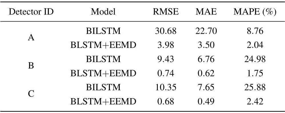
Table 5. Comparison of traffic flow data prediction among detectors(A,B,C).

3.4.5. Traffic flow data prediction on different time scales for detector A

In order to verify the effect of the model on the long-term traffic flow prediction, we use the model to predict the traffic flows in different time spans,i.e., 5 min, 10 min, 15 min.we use the mainline data (detector A) to predict the traffic flow. The results are shown in Table 6. It can be observed that with the increase of time span,RMES,MAE,and MAPE all become larger. This is because with the increase of time span, the data sampling frequency turns smaller, resulting in greater noise in the sampling data,and some characteristic information of traffic flow may be confirmed. Therefore, the error of prediction results will increase. The results show that EEMD+BILSTM has the best prediction effect,the RMSEs of EEMD+BILSTM for 10 min and 15 min are 8.95 and 15.36, respectively. The prediction trend of wavelet denoising and EEMD de-noising are also consistent with that of EEMD+BILSTM. The results show that the model can also achieve good long-term forecasting results,and the model can be used for long-term prediction.

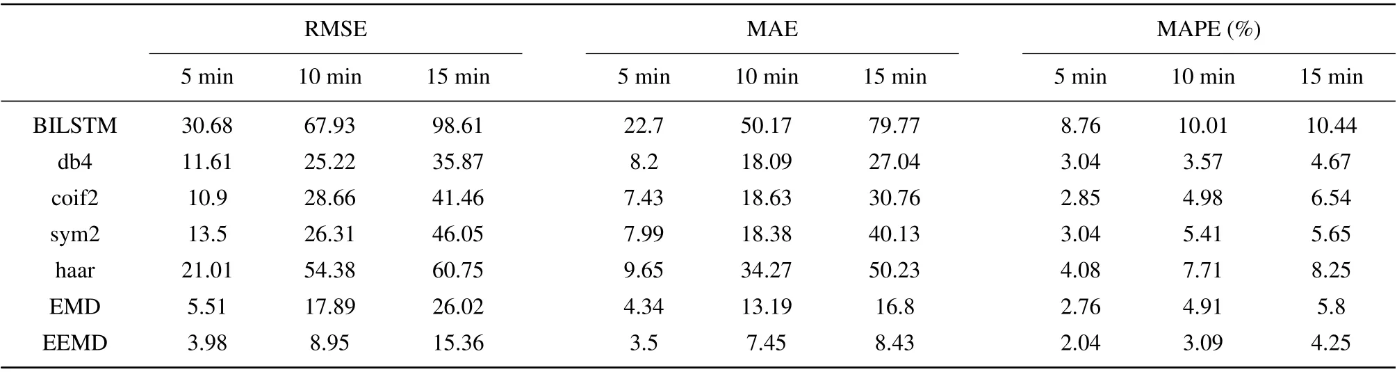
Table 6. Statistical performance on different time scales for detector A.

4. Conclusions

In this study a novel traffic flow prediction framework is introduced by integrating a data denoising scheme with a deep learning model. This study adopt the traffic volume data collected from three detectors in San Diego, California, which are cited from the PeMS. To clean the data, we employ various popular and effective noise reduction models to suppress outliers from the raw traffic flow data. We chose three denoising schemes: EMD, EEMD, and Wavelet with different basis (haar, db4, sym2, coif2). Then combine with BILSTM to make predictions. Finally, we compare the prediction accuracies of different models by analyzing the RMSE, MAE,and MAPE indicators. Several interesting conclusions can be summarized as follows.

(I) The model combines the data denoising with the model, which is better than the prediction process of without denoising strategy.

(II) The performances of WL (db4), WL (coif2), WL(sym2) are better than that of WL (haar). In addition, the performance of WL (haar) in long-term prediction is not so satisfactory as other three wavelet methods.

(III)The BILSTM+EEMD obtains the best performance in comparison with all the WL models and BILSTM+EMD.The RMSE,MAE,and MAPE indicators of BILSTM+EEMD are all at least 25%lower than those of other methods.

(IV) These hybrid forecasting methods can be used in long-term prediction. The model proposed in this paper can make the prediction more accurate. It can be used to optimize traffic organization strategy,improve traffic efficiency,and reduce energy consumption.

(V)In future,there will be several directions for more indepth study. Firstly, this paper has no predictive influence of environmental factors on the forecast,which can be taken into account later. Secondly, we can take some traffic indicators into account in traffic flow prediction,such as speed and road occupancy. Finally, we can combine deep learning with traffic flow models (e.g., car-following models) to predict traffic flow.

Acknowledgements

Project supported by the Program of Humanities and Social Science of the Education Ministry of China (Grant No. 20YJA630008), the Natural Science Foundation of Zhejiang Province, China (Grant No. LY20G010004), and the K C Wong Magna Fund in Ningbo University,China.