The intermittent excitation of geodesic acoustic mode by resonant Instanton of electron drift wave envelope in L-mode discharge near tokamak edge

Zhao-Yang Liu(刘朝阳) Yang-Zhong Zhang(章扬忠) Swadesh Mitter MahajanA-Di Liu(刘阿娣) Chu Zhou(周楚) and Tao Xie(谢涛)

1Institute for Fusion Theory and Simulation and Department of Physics,Zhejiang University,Hangzhou 310027,China

2Center for Magnetic Fusion Theory,Chinese Academy of Sciences,Hefei 230026,China

3Institute for Fusion Studies,University of Texas at Austin,Austin,Texas 78712,USA

4School of Nuclear Science and Technology,University of Science and Technology of China,Hefei 230026,China

5School of Science,Sichuan University of Science and Engineering,Zigong 643000,China

Keywords: zonal flow,drift wave,Instanton,L-H mode

1. Introduction

Zonal flows are ubiquitous in nature and in the laboratory.[1,2]In a plasma torus like tokamak they appear in two distinct manifestations: the toroidal low frequency zonal flow(TLFZF)and GAM.The latter,usually,is observed as ‘intermittent excitation’,[2]that does not persist. Though the existence of intermittent excitations has been reported in many simulations,[3-6]no physical mechanism has been clearly identified. There are many theories for GAM onset,but none of them would lead to an intermittent excitation until recently.[7]In that paper we proposed and hopefully showed that the Caviton to Instanton transition, developed in a previous paper[8]for drift wave-zonal flow system,may trigger the ‘intermittent excitation’ of GAM for ambient ITG turbulence. One may wonder if what the situation would be for ambient turbulence in the electron direction. The present paper is prepared for answering this question. It is not simply to reproduce the procedure in Ref.[7]which has already adopted many results derived in Ref. [8]. Instead, the present paper is essentially self-contained in a sense that it begins with the multi-scale manipulation for mode in electron direction; containing both micro-scale and meso-scale equations. On the other hand,more details regarding the motion of Caviton and Instanton are explored and analyzed;leading to the conclusion that GAM is excited by resonant Instanton.

One must confront at the outset that the best-known drift waves in the electron direction - namely the collisionlesstrapped electron mode (CTEM or simply TEM) and dissipative-trapped electron mode (DTEM)[9,10]- are not likely to be major constituents of the L-mode turbulence because of high collisionality in the edge region where GAM activity is observed(see Appendix A of Ref.[7]),however,TEM and DTEM have been reportedly observed in I- and/or Hmode.In this paper,we will resort on the instability associated with the relatively simple but well-knownδe-model;[11-13]it will be examined as a candidate for edge turbulence. We choose this model for its relative simplicity,even though more realistic models, such as impurity-driven drift waves, do exist in literature.[14]Notice that the description of the latter requires the simultaneous treatment of several fields: the perturbed density, temperature, and parallel velocities for electrons,main ions,and impurities. A two-dimensional(2D)theory(for example,in the 2D ballooning representation)for such a system is quite complicated. No doubt that these complexities could be significant, but a first attempt with a simpler model is quite appropriate. We expect that the fuller models may be essential to predict linear growth rates and marginal stability criteria,but quantities like Reynolds stress and group velocity (determined by the structure of the mode potential)may be well approximated in the simpler model. The last but not the least reason for the simpler approach is that a lack of experimental knowledge on impurities (at the L-H transition threshold) would be a serious impediment to the analysis of the impurity driven mode. For brevity, the toroidal electron drift wave inδe-model will be calledδe-mode.

In this paper, theδe-mode will be treated as a 2D system. In order to obtain the 2D structure of the mode it is important to keep all the translational symmetry breaking(TSB)terms.[13,15]When TSB terms are neglected,the resulting 1D equation yields two branches: the slab-like Pearlstein-Berk branch[16]stabilized by the magnetic shear,[17,18]and the Chen-Cheng branch,[12,19]an intrinsic toroidal branch that disappears in the slab limit. For the latter branch the shear stabilization is greatly reduced owing to ‘tunneling’;[12]consequently the finite non-adiabatic part of electron density can render the mode unstable. The growth rate of the latter branch is, likely, greater than the former one for sameδe. Therefore,in this paperδe-mode solely refers to the intrinsic toroidal branch.

The remaining part of the paper is organized as follows.In Section 2 the multiple scale derivative expansion method in spatiotemporal configuration is applied toδe-mode. In Section 3 the micro-scale equation is solved by making use of the 2D WABT.[15]The solution is then chosen to be the initial guess of an iterative finite difference method to acquire more accurate results in Section 4. Use is made of the two types of solutions to obtain the spatiotemporal structure of Reynolds stress and group velocity in Section 5. This sets the stage for substituting the principal ingredients into the drift wavezonal flow equations (37) and (38), which do not contain the high frequency branch - GAM in zonal flow equation. The information regarding Instanton is given in Section 6. Section 7 begins with introducing the zonal flow equation containing the high frequency branch - GAM for EDW in existing literature. It is followed by two sub-sections. The causal relationship of GAM excitation to Instanton frequency is depicted in Subsection 7.1 for GAM pertaining to single central rational surface. In Subsection 7.2, the intermittency is explained by nonlinear coupling between multiple central rational surfaces. We will show that this coupling introduces the random phase mixing between multiple central rational surfaces in the reaction region,which leads to the intermittency of GAM excitation. Discussion and conclusions are given in Section 8.

2. Multiple scale derivative expansion method for δe-mode

Theδe-mode of this paper is built on a large-aspect-ratio,up-down symmetric tokamak equilibrium with concentric circular magnetic surfaces. We start from the first two linear moment equations - the continuity equation of warm ion fluid, and ion parallel momentum equation under modulation of zonal flow

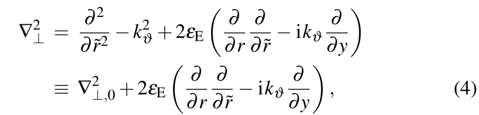
where ˜t,˜r(t,r)denotes fast(slow)scale variables(in toroidal coordinater ≡(r,ϑ,ζ),corresponding to the radial,poloidal,and toroidal directions respectively),εE≪1 is introduced for bookkeeping. Theδe-mode potentialφ(˜t,˜r) varies on fast scale (usually with high frequencyω:φ(˜t,˜r) =φ(˜r)exp(-iω˜t)), while the drift wave envelope ¯φ(t,r)which is modulated by zonal flow ¯υhas slow variation. The zonal flow in slow scale is treated to be small quantity, ¯υ·∇→εE¯υ(∂/∂˜y). Herey ≡rjϑand∂/∂˜y →-i(m+l)/rj ≈-ikϑ,kϑ ≡m/rj(negative in this paper),m(l)is the central(sideband)poloidal number andrjdenotes the position of rational surface.The differential operators of interest,calculated to orderεE,are

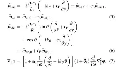
Substituting Eqs.(4)-(7)into Eq.(1)yields

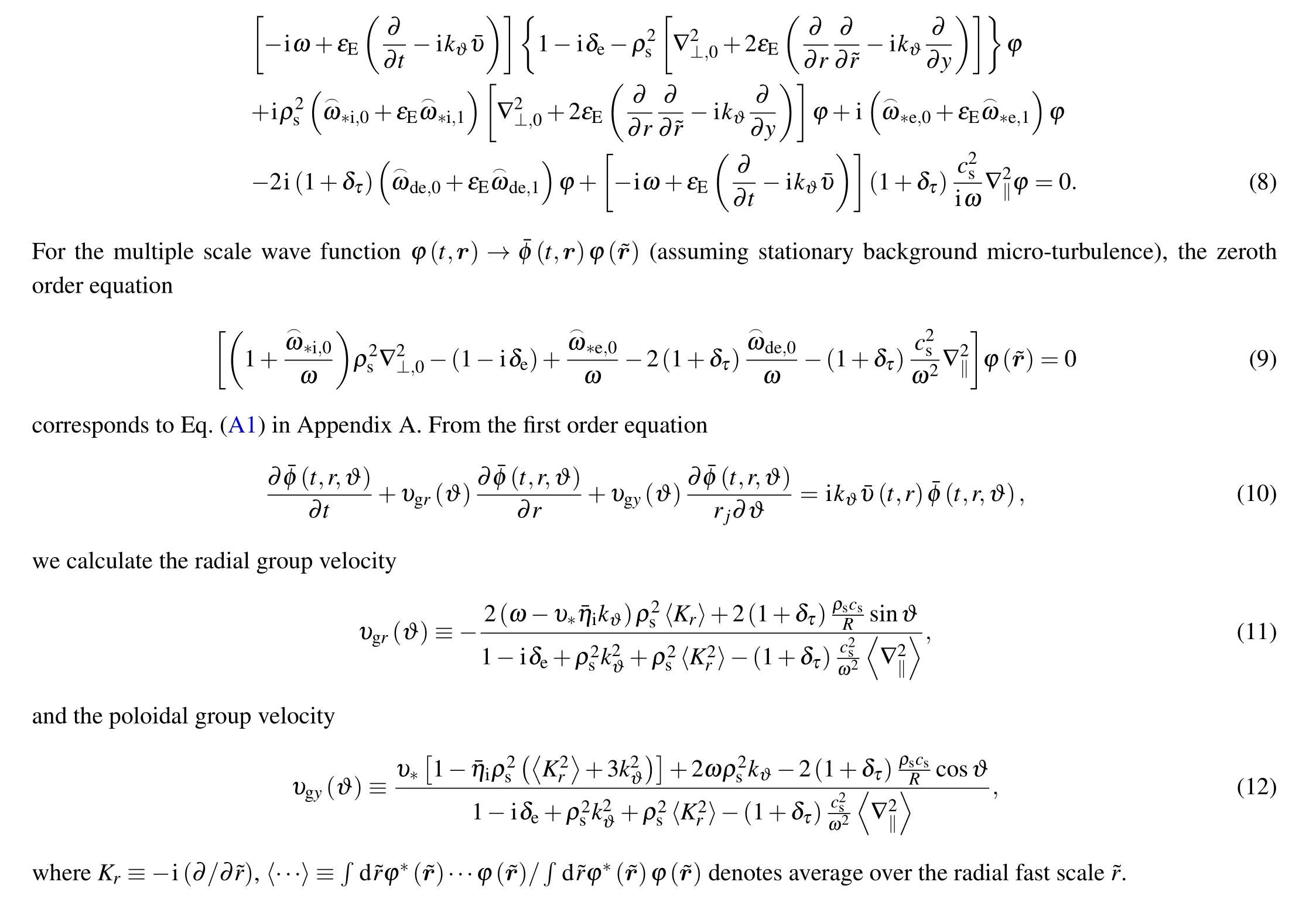
Before ending this section it is appropriate to point out that the explicitly different notation for two different scales makes sense only for derivative expansion in a singular perturbation theory. Such distinctions(˜r˜t)will not appear in the rest of the paper.

3. WABT for solving δe-mode

In the toroidal coordinates(r,ϑ,ζ),the two-dimensional mode can be expressed in the(x,l)representation near the rational surfacerj

wherenis the toroidal mode number(a good quantum number in this paper),m=nq(rj)is the poloidal mode(integer)number,qis the safety factor of the tokamak. The rational surfacerjis called central rational surface of the local mode,uniquely defined by the pair of integers (n,m) and monotonicq(r) to make it distinctive to other rational surfaces contained in the local mode(called sidebands). The(x,l)is a prestigious representation for studying the toroidal modes localized at central rational surfacerj, including multiple sidebands. The extendedδe-model,[11-13]including the translational symmetric breaking(TSB)terms, comes from the zeroth order equation (9). In (x,l) representation, wherex ≡kϑˆs(r-rj) and ˆs ≡d lnq(rj)/d lnris the magnetic shear,it reads

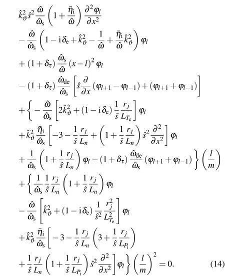
Equation (14) is derived in Appendix A, where ˆkϑ ≡ρs,jkϑ, ˆω ≡ω/ω∗e,j, ˆωs≡cs,j/qRω∗e,j, ˆωde≡ωde,j/ω∗e,j,subscriptjdenotes equilibrium quantities on rational surfacerj, the electron (ion) diamagnetic frequencyω∗e≡-kϑT(0)e/eBLn(ω∗i= ¯ηiω∗e) and the curvature frequencyωde≡-kϑT(0)e/eBR,Ris the major radius,Bis the equilibrium magnetic field,Ln,LTeandLPiare the density, electron temperature,and ion pressure gradient length respectively,andeis the unit electric charge. The remaining part of this section will be written in such a manner that is more accessible to readers who are not familiar with WABT and/or the 2D ballooning theory;some known facts may need to be repeated for better readability.

For a highnlocal mode pertaining to a given rational surfacerjthe monotonic safety factorq(r)can be expanded up to the first order:q(r)≈q(rj)+(dq/dr)(r-rj)≡q(rj)+x/n.Then, one may develop the 2D theory by invoking the 2D Fourier-ballooning transform[13,15,21-23]For WABT,we may assumeφ(k,λ):=ψ(λ)χ(k,λ),whereψ(λ)is a fast varying function inλ,known as Floquet phase distribution(FPD),χ(k,λ)is the solution of ballooning equation (parameterized byλthroughsinλand cosλ).ψ(λ) is localized around someλ∗. In the limitψ(λ)→δ(λ-λ∗)(δdenotes Dirac delta function),equation(15)reduces to the Lee-Van Dam representation.[24]Notice that equation(15)is the mathematical transform (the inverse transform does exist and unique). The 2D ballooning equation for theδe-model in WABT is expanded to the second order ofεB≡(1/n)(d/dλ)

is, traditionally, called the ballooning equation withΩ(λ)representing the(λ-parameterized)effective local eigenvalue.The ballooning equation has two salient features: (i) its counter-part in the (x,l) representation (calculated after removing all TSB terms from Eq. (A4) such asl/m →0 andf(x)→f(0)) is translational-invariant under the transform(x,l)→(x+1,l+1), and (ii) the combined parity (CP) conservation,exhibited inL0(k,λ; ˆω)=L0(-k,-λ; ˆω)forces the“eigenvalue”Ω(λ)to be an even function ofλ.

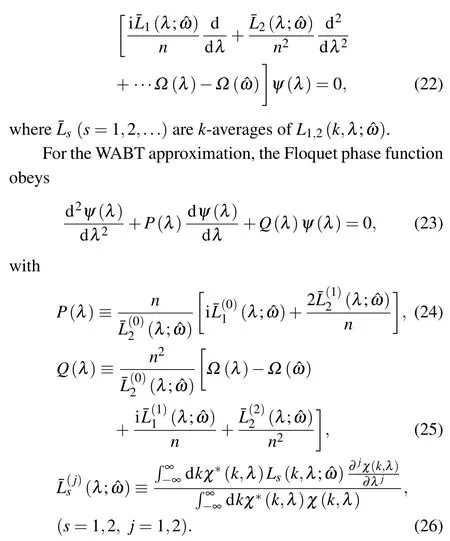
Substituting the solution of Eq. (21) into Eq. (16), and taking average over the first ballooning variablek, yields the differential equation governingψ(λ)(the 2D system is being solved in a series of two 1D equations)

For the numerical calculation, we will use the edge parameters corresponding to an L-mode discharge in the DIII-D tokamak,[25]the basic equilibrium parameters are listed in Table 1(whereR(a)is the major(minor)radius of tokamak,Ln(LTe) is the density (electron temperature) gradient length,B,q, ˆs,ne,andTeare the equilibrium magnetic field,safety factor, magnetic shear, electron density, and temperature at the position of rational surfacerjrespectively,τiis the ratio of ion to electron temperature).

At largek, the ballooning equation (21) becomes a Weber-Hermite equation allowing the asymptotic boundary condition for an outgoing wave[16]

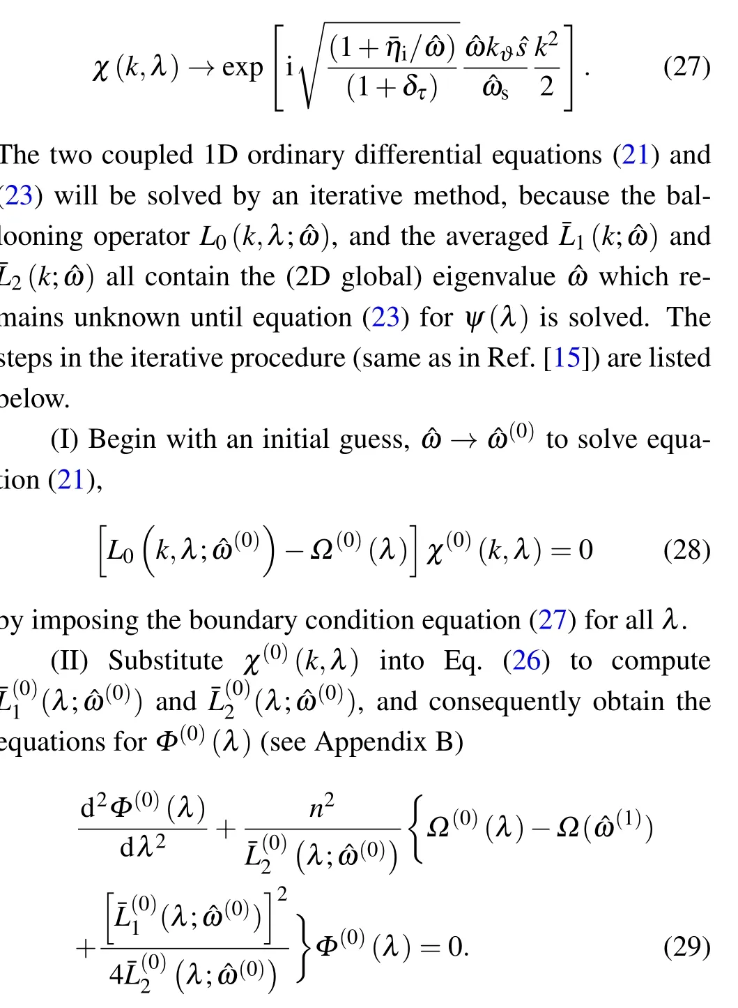
This equation is solved with evanescent boundary conditions.

(III)The global eigenvalue ˆω(1)follows from Eq.(17)by substituting the eigenvalue of Eq.(29)Ω(ˆω(1)).

Repeat the procedures(I)-(III)to obtain ˆω(i+1)from ˆω(i)until|1- ˆω(i+1)/ˆω(i)|＜εwithε ≡10-4as the convergence condition.

Table 1. Basic equilibrium parameters.

The Floquet phaseψ(λ)is shown in Fig.3. The real part ofψ(λ)is Gaussian located atλ=0. The imaginary part looks like a dipole with two peaks aroundλ=±0.74 and breaks theλ-inversion symmetry(resulting from the small parameterΞ).

Fig.1. Potential structure V(k,λ)and wave function χ(k,λ)at(a)λ =-0.74,(b)λ =0,and(c)λ =0.74.

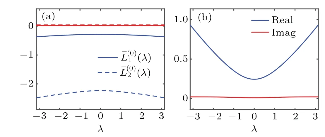
Fig. 2. (a) Average higher order coeffciient (λ),(λ), (b) local eigenvalue Ω(λ).

Fig.3. The Floquet phase distribution(FPD)ψ(λ).

4. Iterative finite difference method for δe mode

In order to expose the spatial structure of theδemode,we must convert the 2D wave functionφ(k,λ)=χ(k,λ)ψ(λ)(obtained in ballooning space) into the (x,l) representation by making use of the 2D Fourier-ballooning transform equation(15),

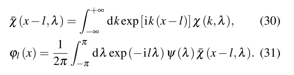
On substituting ¯χ(x-l,λ)into Eq.(31)and integrating overλ, we get the WABT wave functionsφl(x) corresponding to the poloidal mode numberl;φl(x) for variousl=-4,-3,...,4,5 are displayed in Fig.4(a).This solution can be used as an initial guess in the shifted inverse power method[26]to solve the 2D eigenvalue problem equation(14)on the(x,l)grid by the iterative finite difference method. In fact, the WABT solution provides not only the radial boundary of each rational surface to be outgoing waves,but also the phase relation between neighboring rational surfaces,as natural boundary condition for the 2D local eigenmode.[27]

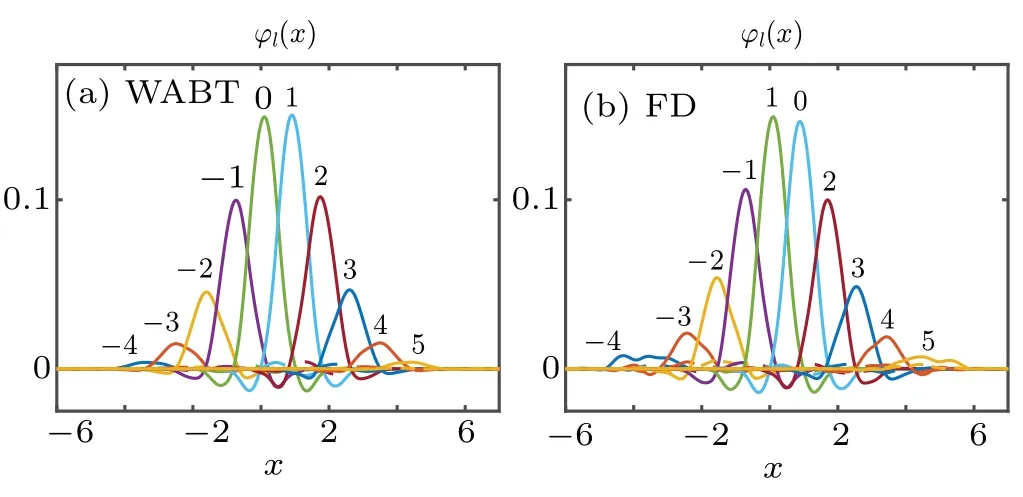
Fig.4.Wave functions φl(x)(l=-4,-3,...,4,5)of(a)WABT and(b)iterative finite difference solution,the solid and dashed lines are real and imaginary parts respectively. The position of central rational surface is shown by x=0. This local mode contains 9 sidebands marked by non-zero l.

The 2D eigenvalue problem equation (14) is put in the form asT[∂/∂x,l; ˆω]φl(x)=Ω(ˆω)φl(x), whereTis a differential operator with derivative ofx, it also depends onland the eigenvalue ˆω. The spatial discrete grids arexk ≡k·h(k=-K,-K+1,...,K-1,K), the step size ish=(xr-xl)/2K,xl(xr) is the left (right) boundary. Thelgrids arel=-L,-L+1,...,L-1,L, andφl(x) is cut-off at large|l|＞L. Use is made of the central difference for derivative ofxto yield the matrix equation

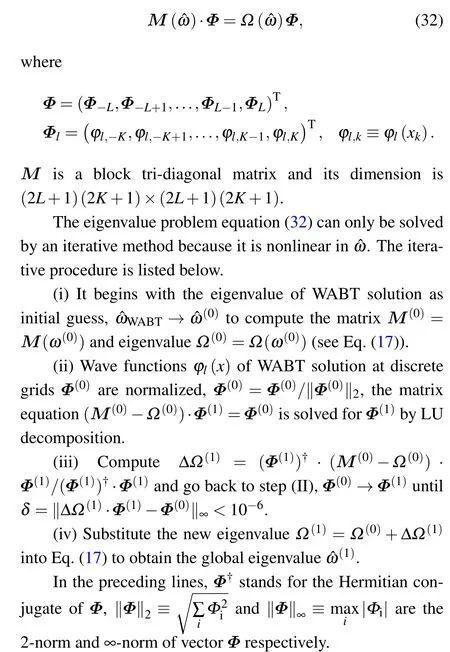
(v) Repeat the Steps (i)-(iv) to obtain ˆω(i+1)from ˆω(i)until|1- ˆω(i+1)/ˆω(i)|＜ε,withε ≡10-4as the convergence condition.

After 5 iterations, the eigenvalue converged to ˆωFD=0.745+0.065i.The difference of iterative finite difference solution and WABT solution,|ˆωFD- ˆωWABT|/|ˆωWABT|≈1.7%,was within the expected error (～1/n=12.5%). The wave functionsφl(x) of the iterative finite difference solution, displayed in Fig. 4(b), are in good agreement with the WABT solution.

The wave function in (r,ϑ) representation,φ(r,ϑ) =exp(-imϑ)∑lφl(x)exp(-ilϑ), is shown in Fig. 5; the 2D mode structureφ(r,ϑ) and the close-up in bad curvature region for both WABT and iterative finite difference solution are highlighted. The mode structure,embodied in the wave function,is the crucial input to compute Reynolds stress and group velocity ofδemode in Section 5.

One may have noticed that the dumbbell radial structure shown in Fig. 5 is consistent with the almost equal height ofl=0 andl=1 in Fig.4,feathering inward shift of the EDW mode structure. The position ofrj=54 cm is equivalent toρ= 0.9. The actual ‘center of mode’ is always less thanρ=0.9 as shown in Fig. 5, implying an inward shift. It is consistent with the results shown in Fig.4. Positive sideband number corresponds to radial shift inward in our convention that the toroidal number is negative. For example, center of mode forl=1 in Fig. 4 is aroundx=1, corresponding to radial shift Δρ=-0.025.

Fig. 5. 2D mode structure φ(r,ϑ) of (a) WABT solution, (b) its close-up in bad curvature regime, and (c) iterative finite difference solution, (d) its close-up in bad curvature regime, where ρ ≡r/a is the normalized minor radius. The central rational surface of the 2D local mode pertaining to is displayed by dashed lines.

5. Reynolds stress and group velocity for δemode

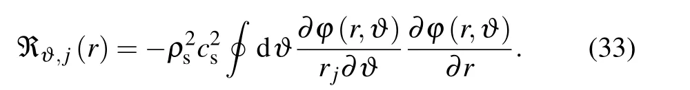
The Reynolds stress is defined by ℜϑ ≡〈˜ur˜uϑ〉, where〈···〉stands for ensemble average, which is equivalent to the average over the poloidal angle.[27,28]For perturbed electrostatic potential ˜u=ρscsb×∇φ, the explicit expression of(poloidal)Reynolds stress pertaining to the rational surfacerjis

The intensity of drift wave forδe-model is defined asIm(r)≡∮dϑφ(r,ϑ)φ(r,ϑ),hereIm(r)describes the radial distribution of drift wave. When computing the physical quantity,we only retain the real part ofφ(r,ϑ).

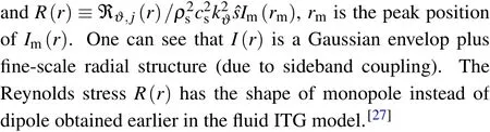
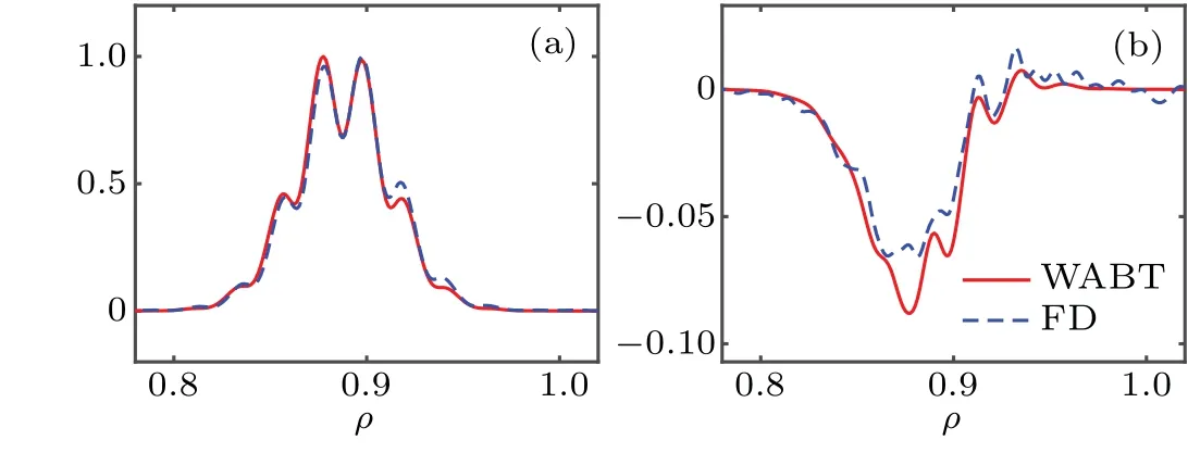
Fig. 6. (a) The intensity of drift wave, (b) Reynolds stress computed by WABT solution(red solid lines)and iterative finite difference solution(blue dashed lines).

The radial and poloidal group velocities are functions only of the poloidal angle because the drift wave in tokamak is a standing wave in radial direction. The characteristic line in poloidal direction of Eq.(10)is given by dϑ/dt=υgy(ϑ)/rj,that yields mapping time to poloidal angleϑ(t). As a result,the radial group velocity becomes a periodic function of time,υgr(t)=υgr(ϑ(t)). To explore the structure of group velocity, the average of three operators over fast scale shown in Eqs.(11)-(12)must be computed:

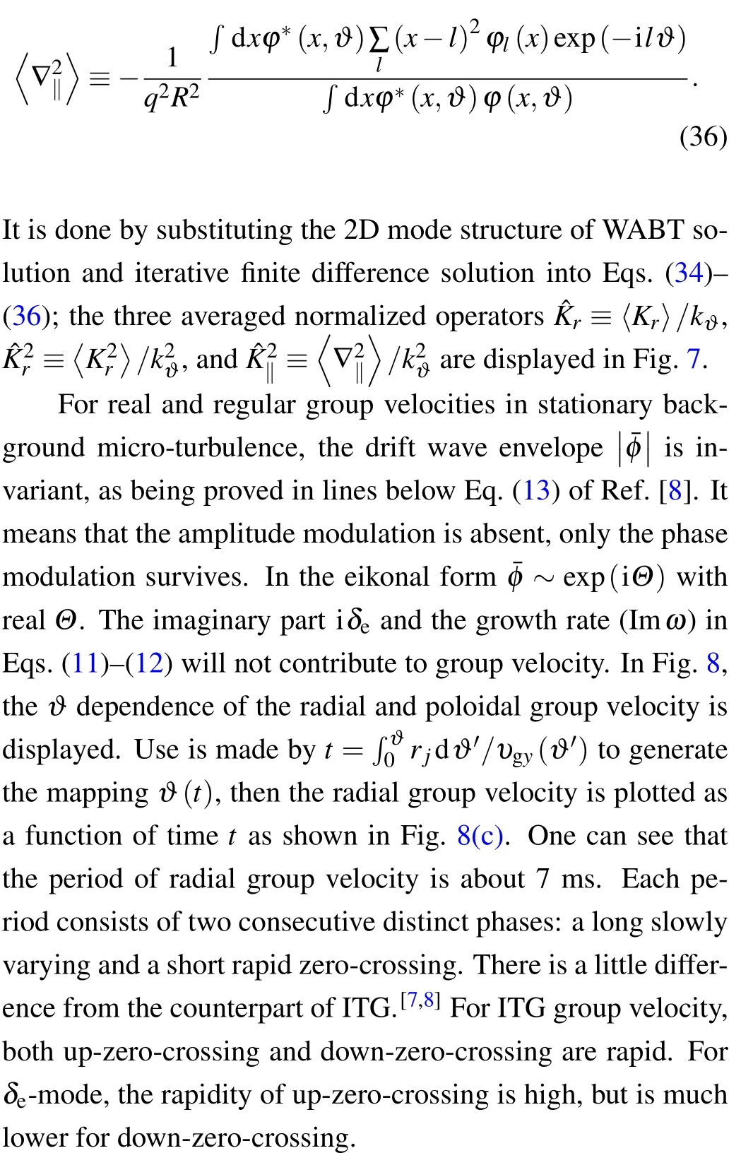
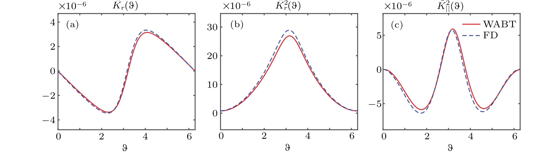
Fig.7. Three normalized operators,(a) Kˆr ≡〈Kr〉/kϑ,(b) ≡ /,(c) ≡/,the red solid and blue dashed lines are solution of WABT and iterative finite difference respectively.

Fig.8. (a)Radial,(b)poloidal group velocities versus ϑ,(c)radial group velocity versus t.

Now, we are ready to study the interplay between zonal flow and phase function in meso-scale provided that the ambient turbulence is EDW.The study is to solve the zonal flow equation and the envelope equation jointly by making use of the Reynolds stress and group velocity obtained in this section for EDW.

6. Remarks on Instanton in δe-mode

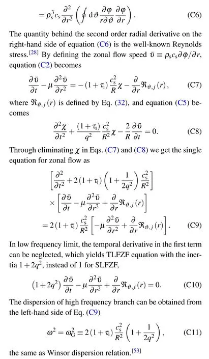
In a torus like tokamak the geodesic curvature introduces high frequency branch into the zonal flow equation via coupling to sound wave. It also modifies the slab low frequency zonal flow (SLFZF) into TLFZF. This has been shown in literature for electron drift wave[29](also see Eq. (C10) in Appendix C).However,the Reynolds stress as the source of zonal flow equation is also modulated by the drift wave envelope,not a static one. It is precisely the purpose of this section to demonstrate that such a modulation plays the key role to intermittent excitation of GAM. The modulation by drift wave envelope is to replace ℜϑ,j(r)by ℜϑ,j(r)cos2Θin the zonal flow equation,whereΘconsists of two phases,[8]because amplitude modulation is absent for drift wave-zonal flow system.A long-lived standing wave phase, which called the Caviton and a short-lived traveling wave phase (in radial direction),called the Instanton. In Caviton phaseΘvaries slowly in time.The corresponding modulation has little impact on the high frequency branch of zonal flow(GAM).Right after the group velocity crosses zero,the Caviton transits to Instanton as a linear traveling wave in radial.Then,it evolves to nonlinear stage rapidly with increasing frequency. As soon as the frequency is resonant to GAM frequency, the GAM is excited. The key processes leading to GAM excitation will be presented in this section.

When the modulation is included in the TLFZF equation in collisional regime given in Refs. [30,31] and Eq. (C10) in Appendix C,it becomes

whereυgr(s)is the radial group velocity of EDW as a function of time,which has been calculated and shown in Fig.8(c). In this section the numerical results are obtained from the solution of Eqs. (37-(38). The numerical results related to GAM excitation will be presented in the next Section 7. The normalization and numerical methods for the zonal flow equation set are introduced in Appendix D and will not be repeated elsewhere.

6.1. Correlation between occurrence of spikes and zerocrossing of radial group velocity

Equations (37)-(38) are numerically solved with parameters listed in Table 1,andIm(rm),the intensity of turbulence,is chosen to be 10-3.

Fig.9. The time evolution of 40 ms for 5 distinct spatial positions to display the relationship of zonal flow kinks,phase spikes and zero-crossing of radial group velocity for Im(rm)=10-3.

The vertical dotted line 1(2)in Figs.9,10 and 14-17 denotes the time point upon downward (upward) zero-crossing of radial group velocity. One can clearly see the huge differences in temporal structure between near zero-crossing and away from zero-crossing. Near zero-crossing structure looks spiky inΘ, kinky in ¯υ; away from zero-crossing structure looks smooth in bothΘand ¯υas shown in Figs.9(b)and 9(c).The similar structures have been shown in Fig.6 of Ref.[8]for ambient turbulence of ITG,where the spiky phase is named Instanton and the smooth phase is named Caviton. The nomenclature can be understood by seeing the spatial structure in Fig.10 of Ref.[8]. The close-up temporal structure ofΘfor 5 radial positions is displayed in Figs. 10(a) and 10(b), very much like that shown in Fig.7 of Ref.[8]. By picking up three radial positions“yellow(ρ=0.90)-red(ρ=0.89)-blue(ρ=0.88)” in Fig. 10(a) one can see a traveling wave moving inward. By the same token,what shown in Fig.10(b)is a traveling wave moving outward. The 3D structures shown in Figs.10(c)and 10(d)depict spatiotemporal structure of EDW envelope square cos2Θin real space. Although the intensity represented by color does not seem accurate to satisfaction (dark region meansΘ=0), it does have roughly shown the locus of the traveling wave; moving inward is shown in Fig.10(c)and moving outward is shown in Fig.10(d). Henceforth, moving inward (outward) traveling wave is referred to be ingoing(outgoing)Instanton.

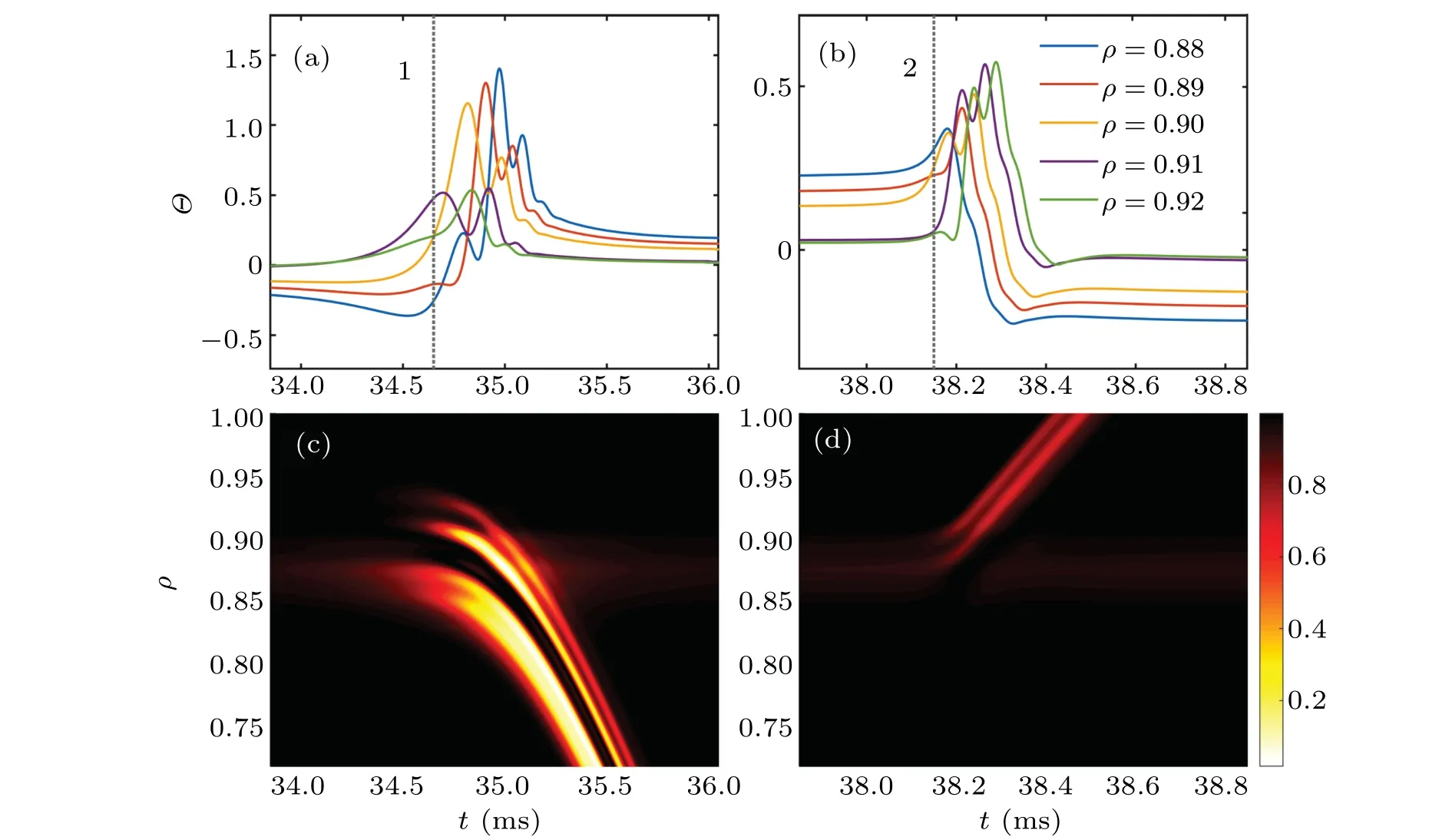
Fig.10. The time evolution of phase Θ and spatiotemporal structure of EDW envelope square cos2Θ near periods 1 and 2 in Fig.9.

6.2. The transition of Caviton to Instanton

The Caviton refers to the phase of drift wave envelope as a slowly moving nonlinear standing wave(smooth phases between spikes in Fig.9(c)). The spatial structure of Caviton is shown in Fig.11 at three moments 33 ms,37 ms,and 40 ms.They look like monopole structure in contrast to the dipole structure for ITG ambient turbulence(Fig.4 of Ref.[8]). The three moments in time are chosen to accommodate two transitions - at 34.65 ms, and at 38.15 ms. The cyan line marks the structure before transition 1. The blue line marks the structure between transitions 1 and 2. The red line marks the structure after transition 2. Apparently, transition 1 alters the negative-Caviton(negative peak)to positive-Caviton(positive peak) and transition 2 alters the positive-Caviton back to negative-Caviton without obvious change in shape. Such a change of spatial structure can also be seen in Fig. 10(a)from 34 ms to 35.5 ms,e.g., the bottom blue line at 34 ms becomes the top blue line at 35.5 ms, similarly in Fig. 10(b)from 38 ms to 38.6 ms. As a rule of thumb the relationship between the sign of the Caviton and zero-crossing is that the downward(upward)zero-crossing leads to positive(negative)sign of Caviton. This rule is valid as long as the sign of radial group velocity remains the same until next zero-crossing occurs(in this paperkϑ ＜0). The spatial structure of Caviton during the period of time when away from the zero-crossing,is approximately determined by radial integration over the zonal flow(υgr(t)[∂Θ(r,t)/∂r]=kϑ¯υ(r,t)),because the time variation of Caviton is small in the envelope equation and can be neglected in that time duration, as shown in Figs. 10(a) and 10(b). As a result,the dipole like zonal flow(the spatial structure of ¯υlooks like dipole as shown by the black dash-dot line in Fig. 13(a) by ignoring details of higher moments) leads to monopole Caviton.

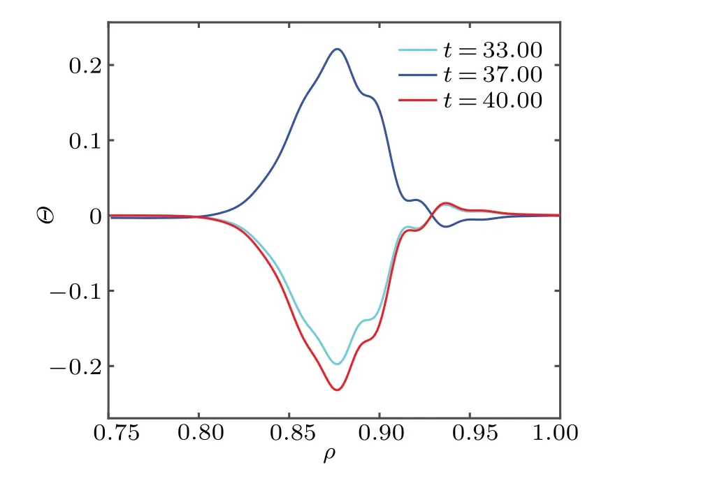
Fig.11. The spatial structure of Caviton at 33 ms,37 ms,and 40 ms.

In Fig.12 displayed is the spatiotemporal structure ofΘaround transitions 1 and 2, where red-black and blue-white represent crest and trough respectively. The travelling waves of ingoing and outgoing Instanton are marked clearly by the strokes in non-green colors. The alternative sign of Caviton is displayed by the change in color within the reaction region,corresponding tor ∈[50,54] cm in Fig.12. The change from yellow to cyan(cyan to yellow)represents the change of positive to negative(negative to positive)Caviton.

Fig.12. The spatiotemporal structure of Θ for EDW.

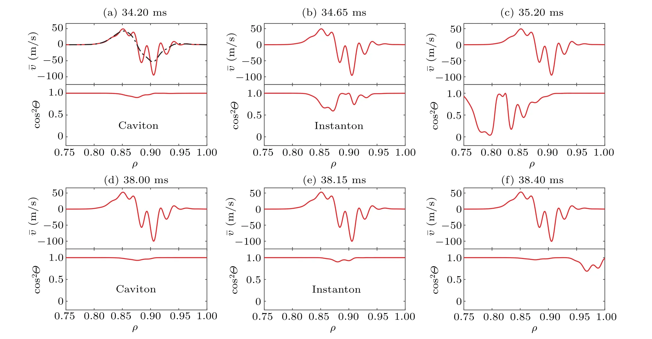
Fig. 13. Snapshots of zonal flow ¯υ and EDW envelope square cos2Θ of 6 time points. The time evolution for 34 ms-40 ms can be seen via the link http://staff.ustc.edu.cn/～lzy0928/spatiotemporal%20evolution.mp4‘spatiotemporal evolution’(Multimedia view).

The transition of Caviton to Instanton can also be presented in the movie ‘spatiotemporal evolution’ in the caption of Fig.13(Multimedia view). This presentation demonstrates vividly that Caviton is a slow nonlinear standing wave and Instanton is a fast traveling wave. Six snapshots of the movie are selected as shown in Fig.13. In Fig.13(a)displayed is the Caviton starts to grow at 34.20 ms fromΘ ≈0. The growing continues until 34.65 ms whenυgrcrosses zero. The early stage Instanton is shown in Fig. 13(b). Then, the ingoing Instanton is shown in Fig. 13(c). One can clearly see that the major portion of Instanton moves outside the reaction region till it totally disappears. In Figs.13(d)-13(e)displayed are the similar process, however, for outgoing Instanton. One may have noticed that the intensity of outgoing Instanton is much weaker than the ingoing one. This is consistent with the intensity shown in Figs. 10(c) and 10(d). It could be attributed to the fact that the lifetime of ingoing(outgoing)Instanton is about 0.55 ms(0.25 ms)due to lower(higher)rapidity of zerocrossing.

Now the general information regarding transition from Caviton to Instanton can be summarized as follows.Before the downward zero-crossing 1 occurs,the eikonalΘis a negative Caviton in shape of monopole. The zero-crossing 1 induces transition from Caviton to ingoing Instanton. As it disappears,a new positive Caviton emerges to grow. It lasts till upward zero-crossing 2 occurs. The zero-crossing 2 induces transition from positive Caviton to outgoing Instanton. As it disappears in reaction region,a new negative Caviton emerges to grow.

Before ending this sub-section, it may be appropriate to briefly describe the physics involving transition of Caviton to Instanton, and the key role played by zero-crossing of radial group velocity.

As shown in Eq. (38), the zonal flow ¯υmodulates drift wave envelope in phase(¯φ～cosΘ,where ¯φis the drift wave

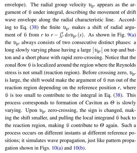
6.3. The nonlinear traveling Instanton with increasing frequency to decades kHz

In this subsection we begin with showing the analytic solution of Instanton near zero-crossing,and compare it with the numerical solution. This study helps us to understand that the spatial structure of zonal flow plays key role in the nonlinear evolution of Instanton, even though it does not change very much during the lifetime of Instanton. We then shall demonstrate that the nonlinear Instanton may evolve to the state containing the spectrum to decades kHz range.

Equation(38)can be cast into the following form:

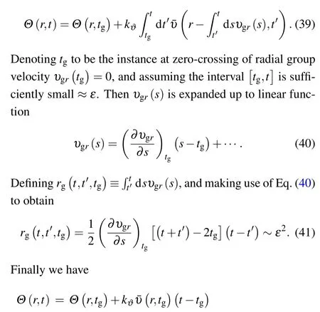
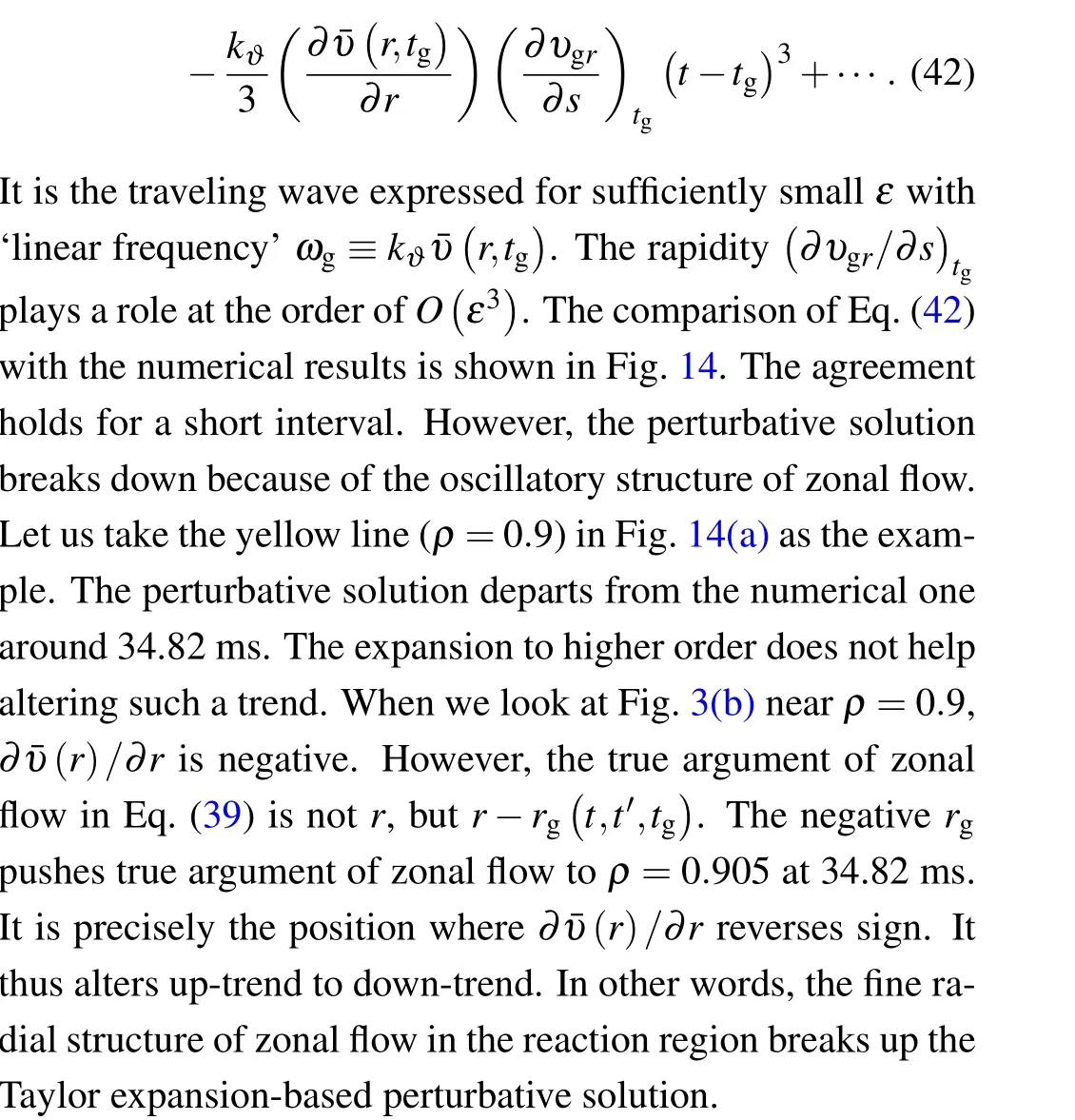
It is also very interesting to see in Fig.14 that at the late stage of Instanton life,say 35.1 ms in panel(a),the lines marking radial position are in the same order as defined by the blue line for Caviton in Fig.11. It implies that the spatial structure of Caviton inherits that generated by the preceding Instanton.

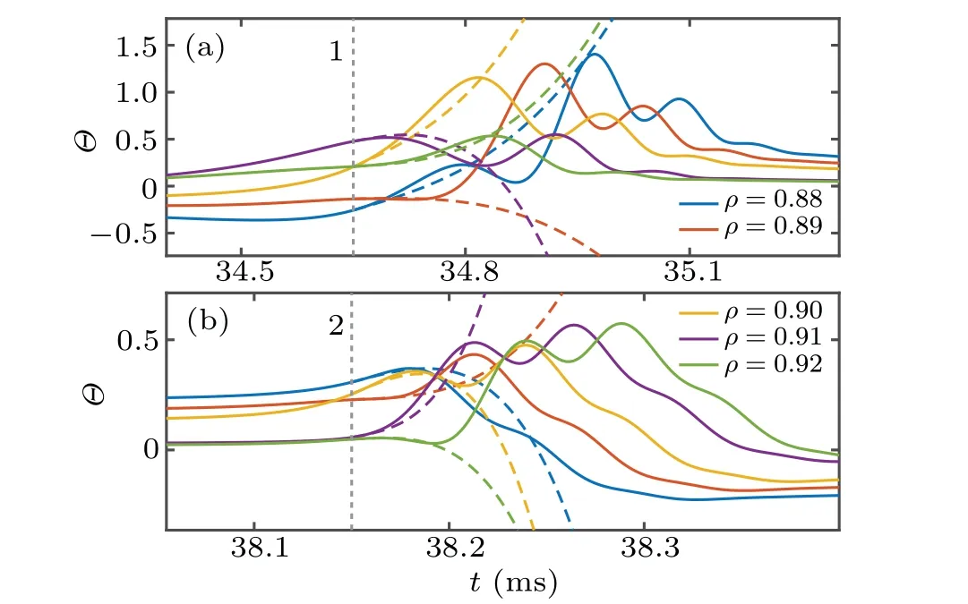
Fig.14. Comparison of analytic results Eq.(42)(dashed lines)to numerical results(solid lines)of Figs.10(a)and 10(b).

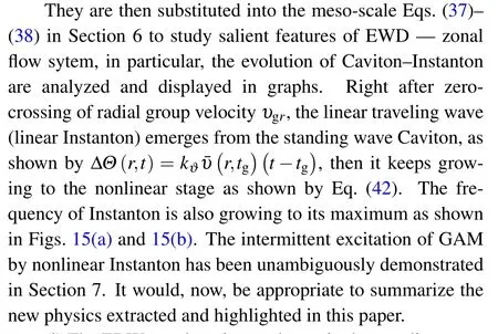
Now,we come to the most important information regarding Instanton,the time evolution of Instanton frequency shown in Fig. 15. It suggests that for GAM frequency in a range of 10 kHz-20 kHz the turbulence level atIm(rm)=10-3is adequate to make Instanton resonant to the GAM frequency,since our numerical results have shown that the maximum of Instanton frequency increases with turbulence level (details are neglected). This implies that static Reynolds stress(no modulation by drift wave envelop)alone does not generate GAM.The causal relationship between GAM excitation and frequency of Instanton will be presented in the next section.

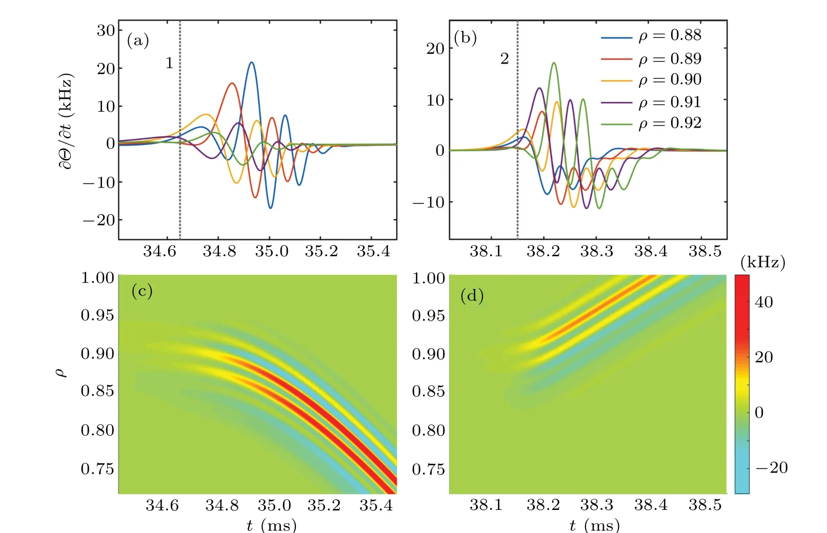
Fig.15. The time evolution of frequency ∂Θ/∂t and its spatiotemporal structure in periods 1 and 2 in Fig.10.

7. The intermittent excitation of GAM by nonlinear Instanton

In order to demonstrate the intermittent excitation of GAM by nonlinear Instanton it is appropriate to use the zonal flow equation derived by Chakrabartiet al.[29]for EDW. In Appendix C the single equation in terms of zonal flow is given by Eq. (C9). Apparently, it is the zero-dispersion equation,and zero propagation. It meansD(τe)=0 in the dispersion relation in Fourier representation[32]

On the other hand, since the EDW envelope is modulated by cosΘ, resulting in cos2Θmodulation to Reynolds stress,equation(C7)should be replaced by

The sound wave equation(45)and the zonal flow equation(46)combined with the envelope equation (38), constitute the basic equation set to illustrate the intermittent excitation of zonal flow by nonlinear Instantons in the next two subsections.They are numerically solved with the same parameters in Section 6 andD(τe)=1 for illustration.

7.1. GAM excitation by nonlinear Instanton for single central rational surface

The time evolution of radial group velocity,zonal flow ¯υand phaseΘare displayed in Fig.16 respectively.

Fig.16. The time evolution of 40 ms for 5 distinct spatial positions to display the relationship of zonal flow including GAM,phase spikes and zerocrossing of radial group velocity.

Comparing with results in Fig.9,one can clearly see that besides the TLFZF defined by Eq.(C10)in Appendix C,a high frequency packet emerges abruptly around the zero-crossing time of radial group velocity. The close-up temporal structure of Instanton frequency∂Θ/∂tand zonal flow in periods 1 and 2 are displayed in Fig. 17. It is apparent that the high frequency zonal flow arises from the rapid variation of the phaseΘ. We have also analyzed results for lower turbulence intensity,e.g.,Im(rm)=10-4(details are neglected),there is almost no GAM excited since the maximum of∂Θ/∂tis around 3 kHz,far below the local GAM frequencyωG=13.64 kHz atρ=0.9.

Fig.17. The time evolution of frequency ∂Θ/∂t and the close-up of zonal flow in periods 1 and 2 in Fig.16.

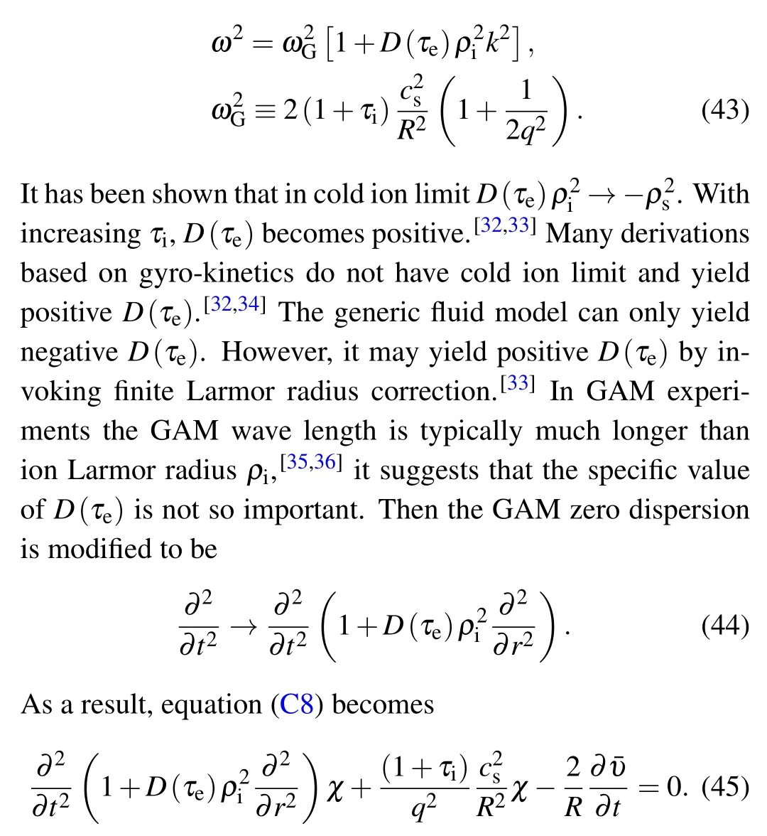
Fig. 18. Spatiotemporal structure of (a) Instanton Im(r)∝cos2Θ and (b) ¯υGAM for D(τe)=1 in period 38.05 ms-39 ms and ρ =0.87-0.94, (c)spectrum versus frequency and spatial position(the red line represents the local GAM frequency ωG),(d)spectrum versus wave number and time.

The excitation of GAM by Instanton is also illustrated in Fig.18 corresponding to period near 2 in Fig.17(d).This is the example that outgoing Instanton induces outward propagating GAM.Among others the wave length of GAM is about 1 cm.It is at the same order of that observed in experiments,[35,36]however,much longer than the ion Larmor radius. It suggests that the spatial structure of Instanton could be more important than the dispersion coefficient in determining the wave length of GAM.

7.2. Nonlinear coupling between multiple central rational surfaces and GAM intermittency

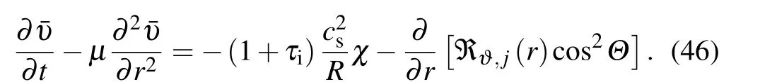
In practice,zonal flow could be driven by nonlinear coupling between multiple central rational surfaces, where the‘coupling’ refers to share of the same zonal flow for each individual central rational surface. For EDW in this paper,there are about 5 rational surfaces within the reaction region(where Reynolds stress in Fig.6 is not small),all of them contribute to a poloidal torque ℜϑ,j(r)(j=0,±1,±2),resulting in the total torque ∑jℜϑ,j(r)cos2Θj. HereΘjrepresents the contribution from thej-th central rational surface. The relative phase between differentΘjis indefinite, because the initial value of integration along the poloidal characteristic line dϑ/dt=υgy(ϑ)/rj, could not be pre-determined in [0,2π].For brevity,this is called random phase mixing between multiple central rational surfaces in the reaction region. It results in the indefinite zero-crossing time of radial group velocity for those rational surfaces shown in Fig. 19(a). As a result,GAMs are triggered asynchronously for different central rational surfaces, forming a rather intricate pattern displayed in Fig. 19(b). Corresponding frequency-time spectrogram is shown in Fig.19(c),very similar to experimental measures of GAM intermittency.[25,37-44]

Fig.19.(a)Temporal evolution of radial group velocity pertaining to 5 rational surfaces,(b)zonal flow at ρ =0.9,and(c)corresponding spectrogram.

8. Summary and on the motion of drift wave envelope

In this paper the full toroidal drift wave - zonal flow system, driven by turbulence associated with an EDW (fluidδe-model), is derived and investigated. By making use of derivative expansion,the two-scale system is constructed. The micro-scale mode structure is solved by making use of 2D ballooning theory,namely WABT.The mode structure is used to calculate two significant meso-scale qunatities in spatiotemporal representation,Reynolds stress,and group velocity.

(i)The EDW envelope is not always in the standing wave(Caviton)phase. Interactions with the zonal flow may lead to the sudden emergence of the short-lived traveling wave in the radial direction (Instanton). This Caviton to Instanton transition,occurring upon the zero-crossing of radial group velocity,is a major event in the evolution of the system.

(ii) The Caviton could be positive (bump) or negative(trough). The Caviton to Instanton transition results in sign reversal,the sign of next Caviton becomes opposite to that of the previous one. The spatial structure of Caviton inherits the radial integration over zonal flow;its sign is determined by the sign of radial group velocity.

(iii) Similarly, there are two types of Instanton, ingoing and outgoing. The ingoing (outgoing) is induced by downward (upward) zero-crossing. It is also associated with the sign of Caviton. The positive (negative) Caviton comes after ingoing(outgoing)Instanton.

(iv)The initial Instanton is a linear traveling wave in radial direction, and, then, it evolves to a nonlinear traveling wave. The amplitude and frequency in the nonlinear stage increases with time initially, it reaches a peak, then oscillates due to the fine radial structure of zonal flow;finally,it falls off because the Instanton travels out of the system.

(v) The maximal frequency of Instanton depends on the turbulence level. For the parameters in this paperIm(rm)=10-3(Im(rm)=10-4),the maximal frequency of Instanton is 20 kHz (3 kHz). Since 20 kHz is high enough to the GAM frequencyωG(13.64 kHz),the GAM is excited by resonance.

(vi) The lifetime of resonance-excited GAM is not long enough to form the ‘WKB eigenmode’.[45]The eigenmode formation would require several times of back and forth reflection between the two boundaries.

(vii) The resonance-excited GAM propagates radially with a wave length much longer than the Larmor radius. This is consistent with observations in experiment.[35,36]

(viii)GAM intermittency follows from the nonlinear coupling between multiple central rational surfaces. The integration along the poloidal characteristics brings in the indefinite initial values pertaining to each central rational surface. It can be called ‘random phase mixing’ between several to decades of central rational surfaces, because the relative phases between the components participating in the coupling are indefinite. For each discharge they are different. Therefore, the pattern as shown in Fig.19(c)is not repeatable.

Appendix A:Derivation of δe-model in(x,l)representation

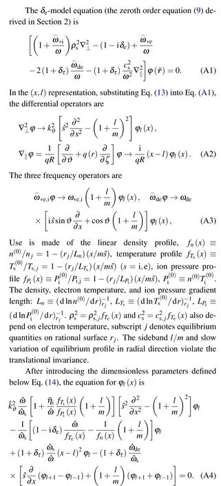
To simplify the derivation,we assume derivatives are applied only on the wave functions,not on the equilibrium quantities, and the TSB termsxin the equilibrium profile can be replaced byl,f(x)≈f(l). Since translational invariance is the leading symmetry, all TSB terms are small enough to be retained up to the second orderO（l2/m2）. Then theδe-model expanded to include TSB terms in the (x,l) representation is obtained as Eq.(14).

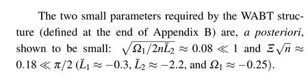
Appendix B:The conditions for valid WABT

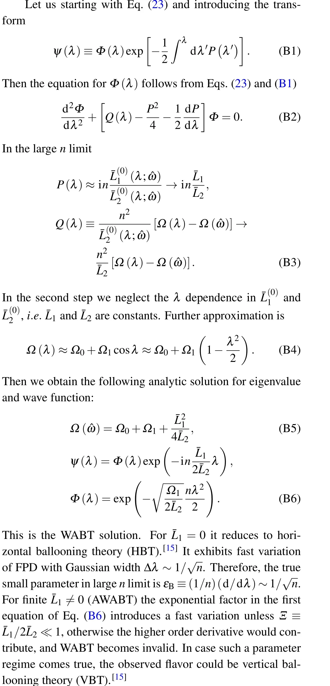
At the end of this appendix, we would like to draw the reader’s attention to the difference between the eigenmode accessible in WABT as distinct from what exists in the literatures, in particular, with the modes discussed in the alternative higher order ballooning theories of authors like Connor-Hastie-Taylor (CHT),[46-48]Dewar,[49,50]and Zonca-Chen.[51]These earlier models create eigenmodes of two very different kinds: (i)the eigenmode is limited to a single position in the radial coordinate,[47,48](ii) or the eigenmode results from applyingad hocboundary conditions at the edge of the domain defined by the equilibrium scales. What WABT,however,is designed to do is neither singular like the first case(coined as isolated mode in Ref.[48])nor dependent upon thead hocvalues of the mode characteristics in the domain which is of little relevance to turbulence. The WABT eigenfunction,though localized at the central rational surface(defined by integersm=nq(rj),m±1=nq（rj±1）,...)covers a finite domain containing rational surfaces atrjof those phase-independent components. What is equally important is that the eigen-structure is dictated by the asymptotic behavior,i.e., natural boundary conditions like evanescence. In some sense the the eigenmode is more spread out than the singular case and much less spread out than the one with boundaries defined on equilibrium length scales. A typical example for the evanescent WABT mode for largekandλ(in the 2D ballooning representation[13,15,21-23]) is shown in Figs. 1 and 3.This is in contrast to the modes built on the equilibrium scale,requiring boundary condition provided by radial equilibrium.The associated mode can only be the global mode within the bounded area,not the local mode pertaining to specific rational surface with natural boundary condition. For a given toroidal numbern, there is only one coherent mode. However, there are many radially adjacent local toroidal modes signified by a series of poloidal numbers (m,m±1,..., statistically independent to each other)corresponding to a givennnumber,just like the multiple central rational surfaces shown in Subsection 7.2; each of the them consists of central rational surface defining parameter of ballooning equation,and multiple sidebands due to TSB terms. In a sense the central rational surface here is very much like the single rational surface in sheared slab model; the only difference is that each one is a toroidal mode not slab mode. The reason for such a discrepancy between the two different types of higher order theories could be traced back to the construction of the lowest order - the ballooning equation. In WABT the ballooning equation is assumed to be translational invariant.[52]As a result, the TSB terms are used to construct the higher order theory in microscopic scale. No similar concept of translational invariance and the broken symmetry (TSB terms) in Refs. [46-51] have ever been introduced.

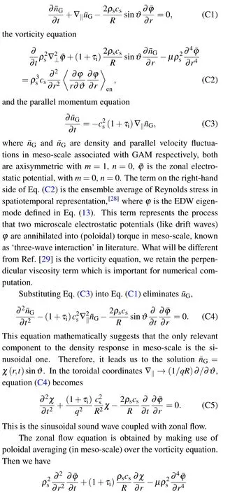
Appendix C: The zonal flow equation for electron drift wave

The zonal flow equation for EDW containing both the low-high frequency branches has been derived in Ref. [29].Since that version is written in Fourier representation, the equations have to be cast into the spatiotemporal representation before being applied to this paper. We shall use the same basic equations,Eqs.(21)-(23)of Ref.[29].They are the governing equations for GAM in dimensional form provided validity of scale separation. The three equations are the continuity equation

Appendix D:Numerical methods for the dimensionless zonal flow equation set

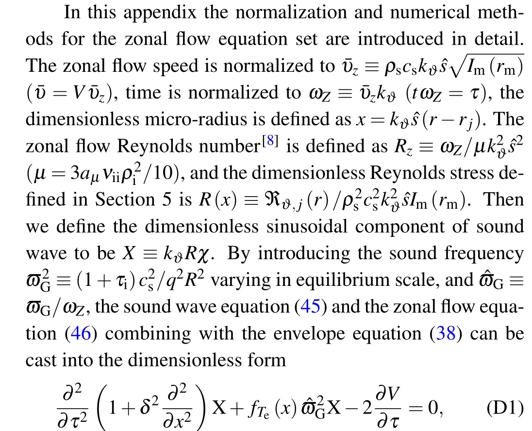
The solution of the initial value problem is worked out for the initial conditions:V(x,0)=0,Θ(x,0)=0,andX(x,0)=0. Since the phase modulation of drift wave envelope is significant only inside the reaction region, the boundary condition for drift wave envelope is not important;the latter is relevant only in the Instanton phase that has a vanishing coupling to zonal flow outside reaction region. However, the signal of phase functionΘcould propagate to a place far away from the reaction region denoted byx±∞,where the cut-off has been introduced(Θ(x±∞,τ)=0).[8]In computationx-∞andx+∞are set to beρ=0.75 andρ=1 respectively.

The boundary condition for the zonal flow equation set has to be set up differently with respect to left and right sides in contrast to Ref. [8], since the data of GAM are measured not too far away from plasma edge,and edge effects on GAM could be important. On the right side, the zero Dirichlet (reflecting)boundary condition is chosen at the plasma edge forV（xedge,τ）=0,χ（xedge,τ）=0, wherexedgedenotes the position of plasma edge(ρ=1),for the reason that GAM cannot propagate outside the last closed magnetic surface. On the left side, an absorptive boundary condition is set up since GAM suffers from Landau damping in lowqregion.[54]

The dimensionless set of Eqs.(D1)-(D3),combined with the assumed initial and boundary conditions, constitutes a well-posed initial value problem, which is solved by making use of the finite difference methods,where the spatiotemporal grids are discretized as (rk,tm),rk ≡r1+k·Δr,tm≡m·Δt,k=0,1,...,Kandm=0,1,...,Mare integers. In this paper we chooseK=600,M=20000,Δr=(r2-r1)/K,Δt=2µs,r1andr2are the positions of the left and right boundaries,corresponding toρ=0.75 andρ=1 respectively. The dimensionless spatiotemporal step sizes are Δx ≡|kϑˆs|·Δrand Δτ ≡ωZ·Δt. Equations (D1) and (D2) are solved by making use of the section order Crank-Nicolson method.[55]The envelope equation(D3)is directly integrated as shown in Appendix C of Ref.[8].

As for the nonlinear coupling between multiple central rational surfaces,equations(D2)and(D3)should be replaced by

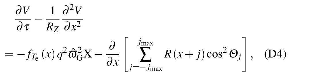
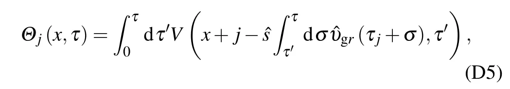
whereτjrepresents the arbitrary initial phase of each rational surface. It is reasonable to assume the mapping between the time and poloidal angleϑ(τj) to be a random number in [0,2π]. Since the interval of adjacent rational surface is Δx=1,the radial argumentxis replaced byx+j.jmax=2 is set for illustration in Section 7.

Acknowledgements

Project supported by the National Natural Science Foundation of China(Grant Nos.U1967206,11975231,11805203,and 11775222), the National MCF Energy Research and Development Program, China (Grant Nos. 2018YFE0311200 and 2017YFE0301204), and the Key Research Program of Frontier Sciences, Chinese Academy of Sciences (Grant No.QYZDB-SSW-SYS004).