A Consistent Time Level Implementation Preserving Second-Order Time Accuracy via a Framework of Unified Time Integrators in the Discrete Element Approach

Tao Xue,Yazhou Wang,Masao Shimada,David Tae,Kumar Tamma,★and Xiaobing Zhang,★

1School of Energy and Power Engineering,Nanjing University of Science and Technology,Nanjing,210094,China

2Department of Mechanical Engineering,University of Minnesota-Twin Cities,Minneapolis,55455,USA

ABSTRACT In this work,a consistent and physically accurate implementation of the general framework of unified second-order time accurate integrators via the well-known GSSSS framework in the Discrete Element Method is presented.The improved tangential displacement evaluation in the present implementation of the discrete element method has been derived and implemented to preserve the consistency of the correct time level evaluation during the time integration process in calculating the algorithmic tangential displacement.Several numerical examples have been used to validate the proposed tangential displacement evaluation;this is in contrast to past practices which only seem to attain the first-order time accuracy due to inconsistent time level implementation with different algorithms for normal and tangential directions.The comparisons with the existing implementation and the superiority of the proposed implementation are given in terms of the convergence rate with improved numerical accuracy in time.Moreover,several schemes via the unified second-order time integrators within the framework of the GSSSS family have been carried out based on the proposed correct implementation.All the numerical results demonstrate that using the existing state-of-the-art implementation reduces the time accuracy to be first-order accurate in time,while the proposed implementation preserves the correct time accuracy to yield second-order.

KEYWORDS Computational dynamics;time integration;Discrete Element Method(DEM)

1 Introduction

In order to numerically describe the behavior of granular materials (not continuous body)represented as a collection of large number of distinct particles,the discrete/distinct element method(DEM),proposed in[1],is being widely used for its ease of implementation and versatility.In the DEM technique,each particle element can undergo large displacement and rotation,and the deformations of individual particle elements are assumed to be small,compared with their displacements;hence we can treat the elements as rigid bodies and the deformation is usually described in terms of the relative normal displacement and the relative tangential displacement between the particles in contact.Consequently,the evaluation of those two displacements has a significant influence on both the dynamic response of particles and the numerical accuracy of the simulation.

One of the common applications for the DEM is particle packing.Various packing methods using DEM have been studied previously such as,Formation of a pile,i.e.,sand piling process[2–6],pouring or depositing particles under gravity[7–12].The DEM particle packing is also used in pharmaceutical field for powder tableting[13,14].Another field of application using DEM is simulating particle flow;and a commonly studied example is ball mill mixer simulation;some of which include,horizontally rotating drums [15–18],tumbling ball mill [19–21].Drum and mill are commonly used in industries for mixing,drying or coating subjects;thus,there is extensive interest among researchers in this study.Besides,the DEM is still studied and utilized in recent studies such as solid-liquid flow simulation[22],impact disruption of cohesive soft sphere simulation[23],granular shear flows of dry flexible fibers[24]and non-spherical complex granular simulation[25].

Furthermore,the DEM not only simulates granular flow,but it can also be used for solid body analysis and assessing fracture as studied in [26].Recently,the DEM has been expanded to be able to solve multi-physics applications where granular particles interact with a continuous body,be it structural or thermodynamics.An Extended Discrete Element Method(XDEM)has been proposed in[27]which couples continuous body analysis method and DEM together without losing small scale information from commonly used volume averaging concept.The XDEM allows those microscale information from particles to accurately influence a macroscopic body.The XDEM opens up a wide variety of possible physical applications in many fields of study.

In transient dynamic simulation of the DEM type problems,contact forces and particle motion need to be evaluated and updated at every time step.The widely used time integrations in the DEM numerical simulations include the explicit Euler method,fourth-order Runge-Kutta(RK-4)method,and central difference method/velocity verlet method,etc.It is straightforward to implement these methods in the DEM simulation;however,these explicit time stepping techniques possess several numerical disadvantages in addition to the conditionally stable features;for example,the Euler methods are first-order accurate in time,RK-4 method requires additional computations of highorder derivatives of differential variables[28,29],and the central difference method is a non-dissipative scheme,i.e.,it cannot introduce numerical dissipation if one needs to.Also,past practices poorly model the tangential physics of particle interactions.Recently,a unified time integration framework,under the umbrella of the so-called generalized single-step single-solve(GSSSS)family of algorithms,including not only implicit,but also explicit single-step single-solve algorithms,which can also be written in a linear three-step form,has been proposed in [30].This single simulation tool kit,which has been originally developed in the field of computational structural dynamics,encompasses not only most existing algorithms that are second-order time accurate and are commonly used over the past 50 years or so,but it additionally inherits a wide variety of new implicit and explicit time integration schemes also with second-order time accuracy,including the explicit central difference method as a special case.To implement these time integrations in DEM and preserve the numerical accuracy of the algorithms,the contact force is required to be evaluated in a consistent way with the selected time integrations in both normal and tangential directions.According to our knowledge,most of the existing literature have been embedding the first-order accurate updating evaluation of tangential displacement into the first/second-order accurate time integrations.The specifics are shown in Section 2,leading to reduced accuracy.

In this work,the main objective is to show the consistent implementation of the GSSSS family of algorithms to the simulation of granular assemblies with DEM while retaining all the advantages of numerous methods within the present framework of algorithms.It is worthy to mention that one major drawback of the DEM technique,as well as the other particle based methods or meshless methods [31–35],is contact detection or neighboring particle search.To circumvent this issue,the linked list is employed to detect the contacting neighbor particles.In addition,Open Multi-Processor(Open MP)is implemented to reduce the simulation computational time.The outline of the rest of the paper is as follows.Section 2 presents the basic theory of DEM formulations and both the linear and the nonlinear model of contact forces and torques are presented in detail.The GSSSS unified time integrators are highlighted in Subsection 2.2 and the specifics of the proposed consistent tangential displacement evaluation is derived and compared with the existing tangential displacement evaluation technique carefully.The effectiveness of the proposed consistent tangential displacement evaluation is demonstrated and illustrated using simple numerical examples in Section 3.Finally,the conclusions are drawn and presented in Section 4.This study shows that the DEM with explicit schemes within the GSSSS family of algorithms achieves and consistently preserves second-order time accuracy;the consistent time level implementation and preserving the second-order time accuracy for the presented results for a wide variety of time integrators in the present unified framework include features such as no overshoot in displacement or no overshoot in velocity or no overshoot in both displacement and velocity for a given set of initial conditions of the particles and differs from algorithm to algorithm.

2 Discrete Element Method with the Explicit GSSSS Family of Algorithms

2.1 Basic DEM Formulations

DEM is a numerical simulation technique for a system of small “distinct” particles/elements,such as powders and granular materials.For the sake of simplicity,we assume the shape of every particle/element in a system is a disk in the two-dimensional Euclidean space E2or a sphere in the three dimensional Euclidean space E3,although DEM can treat any shapes of elements in general,see[36].In DEM,we assume that each particle isrigid,i.e.,no deformation;however,particles are allowed tooverlapslightly one another at the contact points.

Let qi(t): [0,∞)→ Rndimdenote the position component vector of theithparticle (i=1,2,···,nele)with respect to the Cartesian coordinate frameB,whereneleandndimdenote the number of particles/elements in the system and number of dimension,respectively.Suppose that theithandjthparticles are in contact at timetas shown in Fig.1a.The overlap(penetration)between particleiandj,which is denoted bynδij∈R,is defined as

whereriandrjdenote the radii of theithandjthparticles,respectively;anddijis the center distance between the particlesiandjanddij:=‖qj-qi‖=is the center distance between the particlesiandj.We assume the overlap is sufficiently small relatively to the particle sizes.If the inequalitydij ＜ri+rjis met,the overlapnδij＞0 occurs;and the contact forces between patriclesiandjare taken into consideration.Define the unitnormalvector between these particles as nij:=‖nij‖=1.The translational velocity component vectors of particlesiandj(at the center points Ci∈Endimand Cj∈Endim,respectively)with respect toBare given as the(total)time derivatives of the position components vectors,i.e.,vi=q˙iand vj:=q˙j,respectively(denotes the total time derivative of「).Letωiandαidenote the angular velocity and angular acceleration vectors of particlei,respectively(fori=1,2,...,nele).Therefore,the velocity at point Pi∈Endim,as shown in Fig.1a,vPi,can be written as vPi=vi+ωi×ri=vi+riωi×nij,where ri=rinij.Similarly,vPj,the velocity of point Pj,can be written as vPj=vj+ωj×rj=vj-rjωj×nij,where rj=-rjnij.Hence,the relative velocity vector at point Piwith respect to point Pjis obtained as

where vi/j:=vi-vjdenotes the relative translational velocities of particleiwith respect toj.Since the projection of vPi/Pjparallel to nijis given as

the projection of vPi/Pjperpendicular to nij,which is obtained by subtractingnvPi/Pjfrom vPi/Pj,can be written as

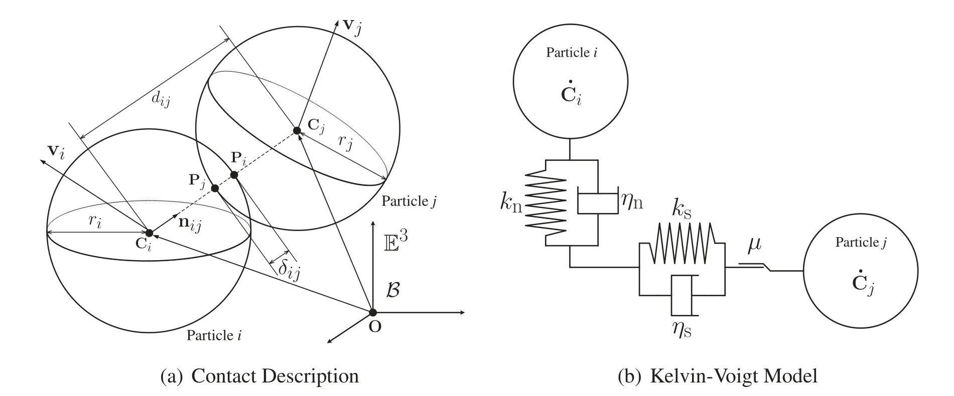
Figure 1:(a) Pictorial illustration of particles i and j in contact;and (b) the Kelvin-Voigt model for particles i and j in contact.O ∈E3 is an origin of a cartesian coordinate frame B for E3 with a righthanded orthonormal basis for the associated vector space

Note thatnvPi/PjandsvPi/Pjare the relative velocity vector of point Piwith respect to point Pjin the normal(nij)and tangential(tij)directions,respectively.Substituting Eqs.(2)into(4)yields:

Hence,tij=

Similarly,we can derive the relative acceleration vectors of point Piwith respect to point Pjin the normal(nij)and tangential(tij)directions.Since the accelerations at Piand Pjare given as aPi=ai+ωi×(ωi×ri)+αi×ri=ai+riωi×(ωi×nij)+riαi×nijand aPj=aj+ωj×(ωj×rj)+αj×rj=aj-rjωj×(ωj×nij)-rjαj×nij,where ai∈Rndim and aj∈Rndim are the linear acceleration vectors of particlesiandj,respectively,the relative acceleration vector at point Piwith respect to point Pjmay be obtained as

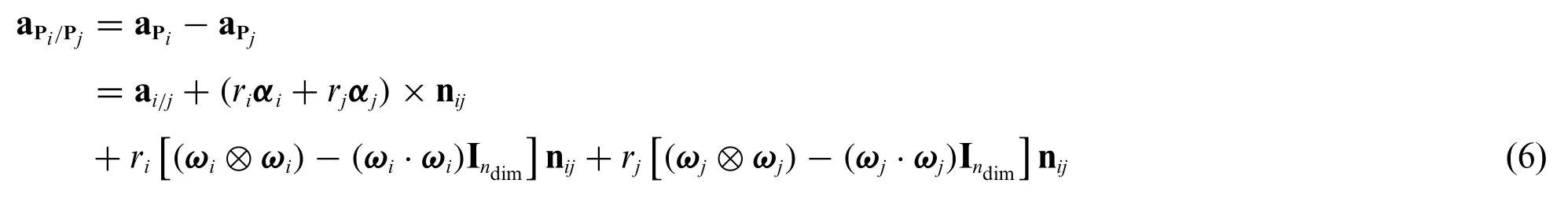
where ai/j:=ai-ajdenotes the relative translational accelerations of particleiwith respect toj,and Indim∈Rndim×ndimdenotes the identity tensor.Hence,the relative acceleration vector of point Piwith respect to point Pjin the normal(nij)and tangential(tij)directions are obtained as

respectively.

Contact Forces and Torques

The resultant contact force and torque acting on particleiare defined as the summations of the contact forces and torques,respectively,acting on particleifrom all particlesj(≠i)that are in contact with particlei.The contact forces due to particle(s)jcan be modeled as follows.

Linear Model:The contact force acting on particleifrom particlejcan be uniquely decomposed into the contact forces in the normal direction(nij)and tangential direction(tij)as fij=nfij+sfij∈Rndim.In DEM,the contact forces are usually modeled by theKelvin-Voigt model,as shown in Fig.1b;hence,both the normal and tangential contact forces on particleidue to particlejhave the stiffness/spring and damping terms,and the friction on the surface is also considered.For the normal contact force,nfij,using the stiffness and damping constants in the normal direction,knandηn,respectively,we have

wherenδijis the relative displacement vector between particleiandjin the normal direction,i.e.,nδij∈Rndim,may be defined as the displacement while the particlesiandjare in contact for the time interval,[tc1,tc2]⊂[0.∞),i.e.,

The viscous damping coefficientηnin Eq.(8)is usually selected asηn=whereCR∈[0,1]⊂R+denotes the coefficient of restitution,and ˆmij,which is sometimes called the reduced mass,is defined as

Similarly,the tangential contact force,sfij,can be written as

whereksandηsare the stiffness and damping coefficients in the tangential direction,respectively.The tangential relative velocity,svPi/Pj,in the equation above is given by Eq.(5).The relative displacement vector between particlesiandjin the tangential direction,i.e.,sδij∈Rndim,may be defined as the displacement while the particlesiandjare in contact for the time interval,[tc1,tc2]⊂[0.∞),i.e.,

We usually takeηs⋍ηnunless otherwise the values of the damping coefficients are critical in the simulation.If the condition||sfij||＞μ||nfij||,whereμ＞0 denotes the coefficient of friction,is met,the“slip”between particlesiandjon the surface at the contact point occurs,and therefore,the tangential contact force,given in Eq.(11),is replaced with the frictional force,sfij=-μ||nfij||tijwithnfij,given in Eq.(8).Once we get all the contact forces,fij,acting on particlei,we can finally obtain the resultant contact force on particleias fi=wherenicontdenotes the number of the particles that are in contact with particleiat timet.On the other hand,the resultant torque on particleican be written in the form

Nonlinear Model:There exist several nonlinear models developed for DEM in the literature to obtain more accurate,realistic simulation results.A common nonlinear model of DEM,proposed in[37],is based on the classical Hertzian contact theory and Mindlin theory[38,39].The normal contact force,nfij,based on the Hertizian contact theory for two spheres,is still defined in the same form as Eq.(8),

However,as opposed to the linear model,nδijand stiffnessknare defined as

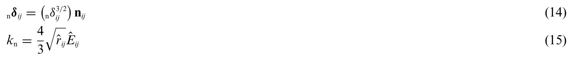
withnδij,defined as in Eq.(1),whereEiandνiare the Young modulus and Poisson ratio of particlei,respectively.For two spherical particles with the same radius (r=ri=rj) and the same material properties (E=Ei=Ejandν=νi=νj),the stiffness defined in Eq.(15)may be written in the form,kn=In the case of a spherical particleiwith a wall,we assumerj→+∞,i.e.,→ri;and thereby,whereEwallandνwallare the Young modulus and Poisson ratio of the wall.According to[37],the normal damping coefficientηnin Eq.(13)is suggested to beηn=in whichis as defined in Eq.(10).Forκ＞0,which can be regarded as dependent on the coefficient of restitution between two sphere particles or between a sphere particle and a wall,it is to be determined empirically by analysts(Usually,α∈[0.01,1]).Note that thenvPi/Pjin Eq.(13)is still defined as given in Eq.(3).

On the other hand,the tangential contact force,sfij,for a nonlinear model is defined,based on the Hertzian contact theory and Mindlin theory[38,39]with the assumption that“no-slip”is allowed between two sphere particlesiandj,as

with

whereGi:=Ei/[2(1+νi)]is called the shear modulus of particlei,andbijis the radius of a contact area between sphere particlesiandj.For two sphere particles with the same radius(r=ri=rj)and the same material properties(E=Ei=Ejandν=νi=νj,i.e.,G:=Gi=Gj),we haveks=In the case of the contact between sphere particleiand a wall,we assume the wall(rj→+∞)is rigid,i.e.,Ej→+∞,since the elastic tangential displacement of the wall due to the contact with particleiis usually negligible;hence,Eq.(17) leads to the following expression:ks=For most applications,we take the same value for the normal and tangential damping coefficients:ηsηn.

2.2 Transient Analysis:A Consistent Time Level Implementation of Unified Time Integrators

Applying the Newton-Euler equation to particleifori=1,2,...,nele,we get

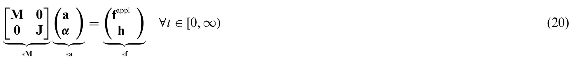
where Mi=miIndim∈Rndim×ndim,with the identity tensor Indim∈Rndim×ndim,and ai∈Rndimdenote the mass tensor and the acceleration vector of particlei,respectively;and Ji∈Rndim×ndimandαi∈Rndimdenote the inertia tensor(with respect to the center of mass)and the angular acceleration vector of particlei,respectively.The right-hand side of Eq.(18),i.e.,fappli∈Rndim,is the applied force on particlei,and it includes any force acting on the particle,including conservative and nonconservative forces,as well as the contact forces described in the previous subsection.Likewise,∈Rndimin Eq.(19)is the applied torque vector of particlei.

In a unified format for all particles (i=1,2,...,nele) in the system,Eqs.(18) and (19) can be written in the form Ma=fappland Jα=happl,respectively,where M=diag(M1,M2,...,Mnele)∈withN:=ndimnele.Or simply,

Time Discretization

Consider the temporal discretization of the governing equations for a time interval I=[t0,tf] ⊂[0,∞)split into subintervals,i.e.,I=[t0,tf]=in whicht0andtfdenote the initial and final time levels of simulation,respectively.The time step size is defined asΔt:=tn+1-tn＞0,and it is assumed to be constant for simplicity.Temporally discretizing Eq.(20)by way of thenormalized time weighted residual methodology[40]results in the following algorithmic framework:

where the algorithmic acceleration,velocity,and configuration vectors are defined as

respectively,forn=0,1,...,f-1.The associated update equations to advance fromt=tntot=tn+1are

The algorithmic parameters,also known as the DNA[discrete numerically assigned]markers,are defined with the input scalar algorithmic parameters(ρ∞min,ρ∞max,ρ∞s),denoting the minimum principal root,the maximum principal root,and the spurious root[41],respectively,together withη,as

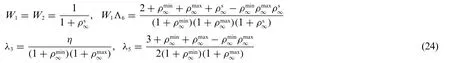
for the U0(ρ∞min,ρ∞max,ρ∞s)family,and

for the V0(ρ∞min,ρ∞max,ρ∞s) family.The U0 and V0 represent zero-order overshooting behaviors in the configuration and the velocity fields,respectively.Note that no two schemes within the algorithmic framework can have the same DNA markers that completely distinguish one scheme from another.Any scheme within this framework is guaranteed to be second-order accurate by approximating*qn≈*q(tn),*vn≈*.q(tn),and*an≈*..q(tn-φ)at the time stepnwhere the acceleration time level shifting parameter is defined byφ:=W1Λ6-W1;see[42]for the details.At timet=t0,the acceleration need to be computed from*a0=*M-1*f(*q0,*v0,t0)where*˜q0=*q(t0)and*˜v0=*.q(t0)are given initial conditions.In DEM simulation,we update fromnton+1 via Eqs.(21)–(23)after evaluating the force vectors,as shown in the previous subsection,at timetn.

Algorithmic Evaluation ofsδij:

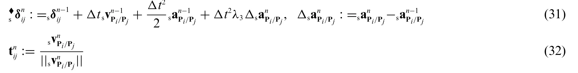
Suppose particlesiandjare in contact during a time interval Ic=[tc1,tc2] ⊂I and split it into subintervals,Ic=[tc1,tc2]=with≡tc2.Following the temporal discretization as given in Eq.(21),the tangential contact force,,is evaluated at q=,v=,andω=.That is,the algorithmic tangential force may be written as

where

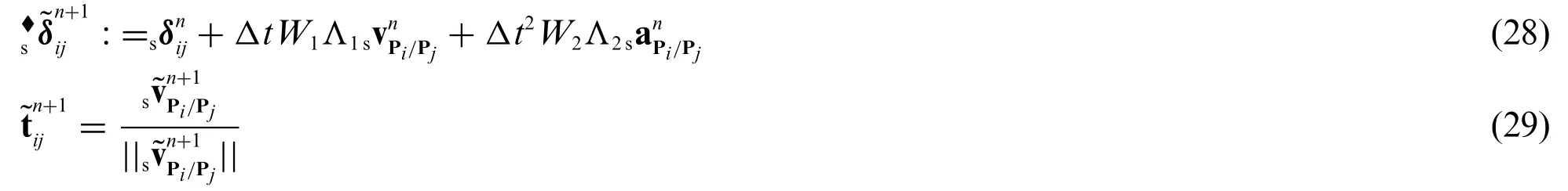
where

Remark

1.If the contact starts at timetn,i.e.,t=tn=tc1,we have=0 in Eq.(28).

3.When slip occurs at the algorithmic time levelin whichis the algorithmic normal contact force defined asand the algorithmic tangential forcedefined in Eq.(26)is replaced with the following algorithmic frictional force,Therefore,the algorithmic tangential displacement vector,,defined in Eq.(27),should be replaced withSimilarly,in the case ofemployinstead of Eq.(30).

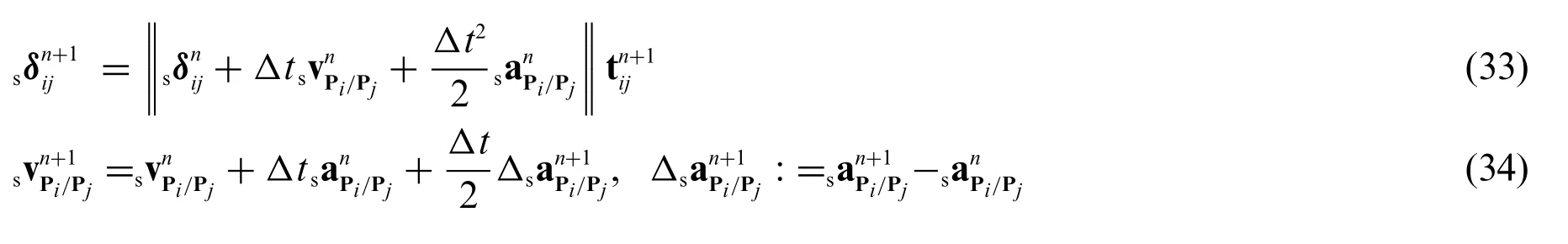
It is worth noting that the tangential acceleration is usually not included during the computations of the tangential contact forces,i.e.,for the central difference method,for example,

is inconsistently used instead of Eq.(33)of the most literature;in this case,the order of accuracy of a scheme within the algorithmic framework presented reduces to only one.

5.For the evaluation of the tangential displacementsδijin Eq.(16)for the nonlinear model in the discrete time system,the approach presented here may be applied in the same manner to ensure the second-order time accuracy of the schemes.

3 Numerical Experiments and Discussion

To verify and validate the concepts described in the previous section,two numerical experiments are given in this section.The main objective of Section 3.1 is to compare the numerical results by traditional tangential displacement evaluation and the proposed consistent evaluation method employing the Central Difference Method.It is worth noting that Central Difference Method is the most widely used explicit second-order time accurate integrator in solving dynamic problems.Therefore,we simply use it as the benchmark in the following simulations.The accuracy in time with different tangential displacement evaluations are given as well.In Section 3.2,a simple 3D granular cube falling problem is simulated with several selected second-order time accurate schemes from the GSSSS unified time integrators.The numerical performances of different schemes with different tangential displacement evaluations are discussed.The linked list algorithm is used to improve the particle searching process and parallel computing is also used in this work.In addition,the calculation time for the 3D case is provided to demonstrate the computational efficiency of the proposed method.

3.1 Validations

To valid our proposed approach and the DEM code,two cases are designed to test the performance of the proposed tangential displacement evolution.Case I is designed to extract the tangential displacement calculation in the general discrete element method.The influence of normal direction is avoided in Case I via fixing a two dimensional disk with only initial angular velocity and constant normal force.Case II gives a general ball falling problem with gravity and the comparisons of traditional and consistent tangential displacement evolution.

Case I:The equation of the tangential motion can be derived to yield a second-order ODE(ordinary differential equation)from Eq.(17),which has an analytical solution for the linear equation.To test our new proposed tangential displacement evaluation method,a very simple and specific physical problem is designed as a 2-D disk with fixed translational movement.As illustrated in Fig.2(left),although the normal force is involved,the tangential movement can be easily extracted.The disk is fixed at the origin O,the initial angular velocityω0is set as 0.5 and the tangential stiffnessksis 1,000.Both the proposed and traditional tangential displacement evaluation method are applied with the central difference method,which has been proved to be equivalent as U0(1,1,0)within the GS4-family,is used in the simulation.

Figure 2:Schematic of the problem.Left:Case I and right:Case II

The comparison of the results with different tangential displacement evaluation methods is given in Fig.3.Both the proposed consistent time level method and the traditional method show good agreement with the analytical solutions in angular position,velocity and acceleration.In this part,our interest is to simply show that the proposed method has the improved or same performance as the traditional method in the sense of capturing physical phenomena.

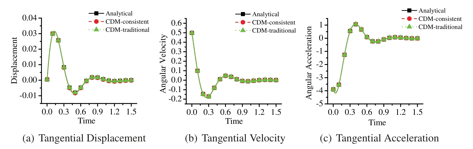
Figure 3:The time history of tangential motion with different tangential displacement evaluation methods

Case II:To complete the validation of our code,a general single ball falling problem shown in Fig.2(right),is simulated by different tangential displacement evaluation methods.To be consistent with the previous numerical simulation case,the central different method is used to solve the governing equation.The time history of ball’s translational trajectory of the center point and rotational motion are given in Fig.4,and the time convergence plots for both methods are given in Fig.5.The top row in Fig.5 provides the convergence plots of position/angular displacement(D),velocity(V),and acceleration (A) evaluated by the central difference scheme with the traditional tangential displacement evaluation method,while the bottom row provides the one evaluated by the GSSSS U0(1,1,0)with the proposed tangential displacement evaluation method.As expected,the results of both methods show excellent agreement as shown in Fig.4.However,as Fig.5(top)shows,the order of convergence in time for the traditional method is only one,in sharp contrast to the proposed method which is of order two.In other words,the well-known second-order accurate central difference method obtains first-order convergence in the case when using the traditional tangential displacement evaluation method.Hence,the superiority of the proposed consistent tangential displacement evaluation over the traditional method is evident with respect to the time accuracy;it also yields improved physics,which can be observed for applications where the tangential effects dominate.

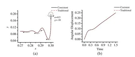
Figure 4:The time history of ball’s motion with different tangential displacement evaluation methods:(a)Translational motion of ball’s center(b)Angular displacement

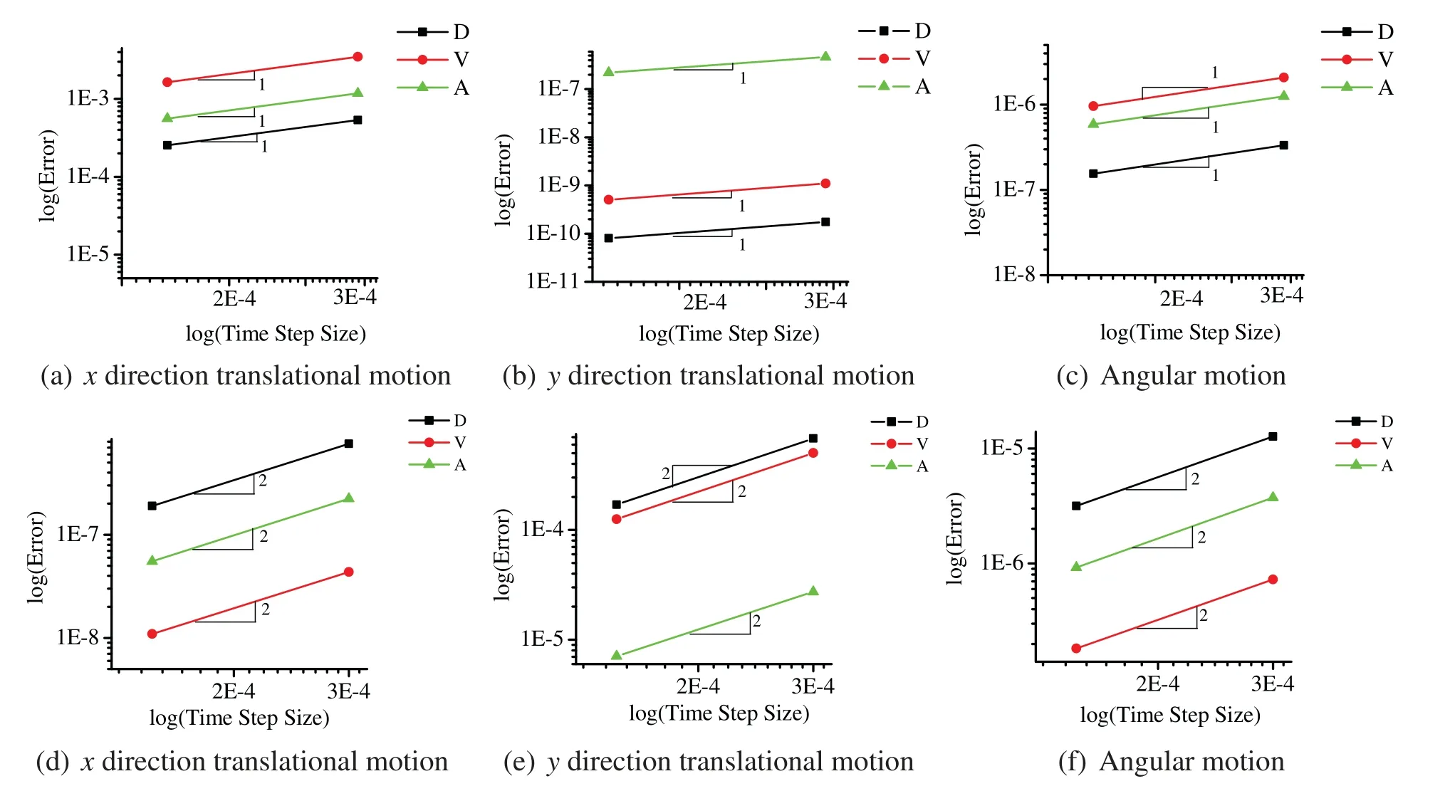
Figure 5:Time accuracy plots of the central difference method with traditional tangential displacement evaluation method(top)and consistent tangential displacement evaluation method(bottom)

3.2 Numerical Experiment

Problem Description:The numerical example chosen in this section is that of a simple granular cube drop of particles in three-dimensional space,as shown in Fig.6.The granular cube has dimensions of 0.3 length×0.3 width×0.3 height,and the container has dimensions of 0.6 length×0.6 width×0.8 height with a cube shape hole(0.2 length×0.2 width×0.2 height)at the bottom.Initially,the particles are packed together and the particle distance(l)and diameter of particles are set to be 0.02,and the total number of particles is 3,375.The mass of each particle is 0.008.The normal and tangential stiffness are chosen askn=1,500 andks=100,respectively.

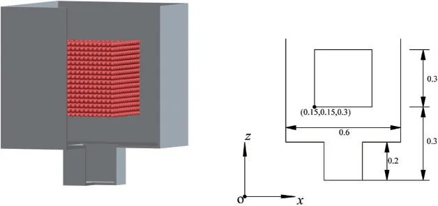
Figure 6:Schematic of the problem(Numerical example)

In this section,the consistent time level implementation and preserving the second-order time accuracy for the presented results in this section are as follows for a wide variety of time integrators in the present unified framework.They yield no overshoot in displacement or no overshoot in velocity or no overshoot in both displacement and velocity for a given set of initial conditions:

· CDM-T:Central Difference Method with traditional tangential displacement evaluation.Note that the central difference method has been proved to be equivalent to the GS4-II U0-based family with(ρ∞min,ρ∞max,ρ∞s)=(1,1,0).

· CDM-C:Central Difference Method with consistent tangential displacement evaluation.

· V0(1,1,0)-C:GS4-II V0-based family with(ρ∞min,ρ∞max,ρ∞s)=(1,1,0)and consistent tangential displacement evaluation.

· U0/V0(0,1,0)-C: GS4-II U0-based family or V0-based family withand consistent tangential displacement evaluation.

Numerical Setting and Computational Cost

In order to capture particle contacts,the time step size used in DEM type simulations is always required to be very small.This implies that the implicit time integration schemes are not necessary in the general DEM simulations.Therefore,in this work,all the schemes listed are explicit and the time step size isΔt=0.0001 within the total simulation duration fromt0=0 totf=2.As mentioned before,the neighborhood particle-detecting process in any particle-based method is the most expensive step in the simulation.In this paper,the linked list algorithm is used to optimize the neighboring particle searching and decrease the computational time,and parallel computing is also applied to improve the computational performance of our code.Our 3D cases were run on a 1.80 GHz,Intel(R)Core(TM)i7-8565K CPU with 8 GB RAM.Table 1 summarizes the specific timings used for all our 3D examples and shows that our proposed GSSSS family of algorithms does not increase computationally cost in comparison to the traditional algorithms,while our proposed method can obtain better computational accuracy(see Fig.5).

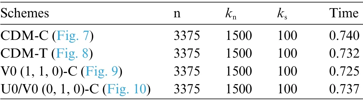
Table 1:Parameters that vary across simulations: n: number of particles,kn: normal stiffness coefficient;ks:tangential stiffness coefficient;Time:average time per 100 time steps

Numerical Results and Discussion

Three-dimensional snapshots with the granular velocity filed values at six different times (t=0.20,0.25,0.30,0.40,0.50 and 1.25)by different schemes are shown in Figs.7 to 10,respectively.The specifics of particle filling process is observed from 0.2 to 0.5 and the final particle distribution is obtained at time 1.25.The process of particle filling the bottom space corresponds to the evolution of total kinetic energy of the system shown in Fig.11(left).As expected,the results of different schemes are very close at each time and the particle distribution shows good physical reliability of the simulation results.In order to better understand the dynamic responses of the granular cube falling process and the computational performance of different schemes,the time history of the total kinetic energy with different schemes are given in Fig.11 (left).Because the central portion of the granular cube keeps charging into the bottom empty space,the total kinetic energy does not decrease immediately,but a short duration (from 0.17 to 0.23) of energy relaxing instead.After the bottom space is filled with particles,the total kinetic energy decreases sharply though some particles on the top layers still keep bouncing.As the frictional force and damping are considered in the particle contact model,the total kinetic energy converges to zero as time goes.

Figure 7:Velocity fields at different time by CDM-C

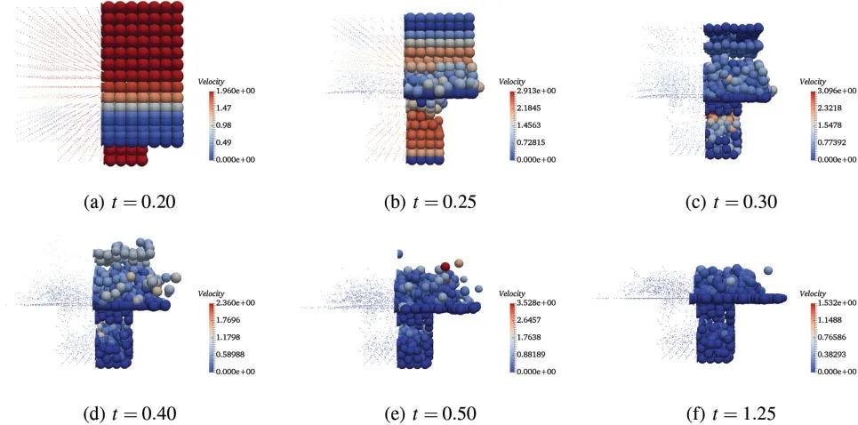
Figure 8:Velocity fields at different time by CDM-T

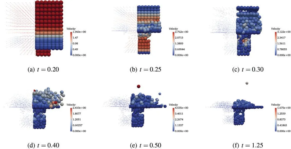
Figure 9:Velocity fields at different time by V0(1,1,0)-C

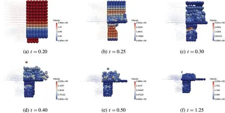
Figure 10:Velocity fields at different time by U0/V0(0,1,0)-C

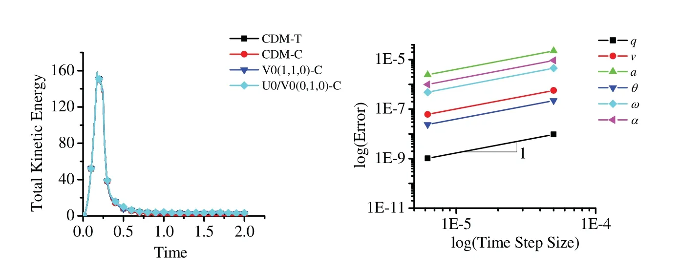
Figure 11:Left: total kinetic energy.Right: time accuracy plots of central different method with traditional tangential displacement evaluation

The time accuracy for translational and rotational position,velocity and acceleration of the central difference method with the traditional tangential displacement evaluation shows only first-order time accuracy in Fig.11 (right).However,alternately,Fig.12 shows the second-order time accuracy for translational position,velocity and acceleration of different time integration schemes selected within the GS4-II family with the proposed consistent tangential displacement evaluation.All the schemes show the second-order time accuracy in both translational and rotational motion.It is to be noted however,that using central difference method in solving the second-order ODE,it is supposed to yield second-order accuracy in time.According to the time convergence order from different tangential displacement evaluations,it implies that the drawback via the traditional tangential displacement evaluation in DEM type method is not at the same time level as the algorithm and has significant influence on the whole system’s time accuracy.In other words,only when the tangential displacement evaluation is evaluated at a consistent time level corresponding to the selected time integration scheme within the unified framework described,the results are completely reliable and the time integration schemes are implemented correctly and efficiently maintaining second-order time accuracy with improvement in physics.

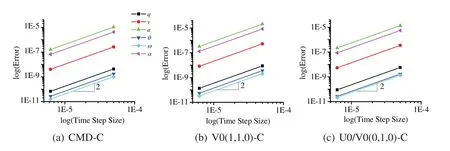
Figure 12:Time accuracy plots of different selected schemes within GS4-II family: q,v and a are translational position,velocity and acceleration,respectively. θ,ω and α are angular displacement,velocity and acceleration,respectively

4 Concluding Remarks

In this work,a consistent tangential displacement evaluation approach is proposed under the framework of the unified second-order time integrators GS4-II family for improving discrete element method (DEM) simulations.The newly proposed approach is derived and designed to maintain the simplicity and generalization of the GS4-II family.Comparing it with the traditional tangential displacement evaluation method,the proposed consistent time level implementation approach can be easily implemented and yields the correct algorithmic tangential displacement at the same time level as in the time integrations via using the same parameters (ρ∞min,ρ∞max,ρ∞s) as the GS4-II family.The improved time accuracy of both the translational and rotational motions by using the proposed method gives second-order accuracy in time,which is consistent with the time integration schemes;whereas,the traditional second-order time integration method such as the central difference can only obtain first-order accuracy in time via using the traditional tangential displacement evaluation.

Acknowledgement: We appreciate all the constructive comments and suggestions from editors and reviewers.

Funding Statement:The authors received no specific funding for this study.

Conflicts of Interest:The authors declare that they have no conflicts of interest to report regarding the present study.