Application of Automated Guided Vehicles in Smart Automated Warehouse Systems:A Survey

Zheng Zhang,Juan Chenand Qing Guo

Beijing University of Chemical Technology,Beijing,100029,China

ABSTRACT Automated Guided Vehicles(AGVs)have been introduced into various applications,such as automated warehouse systems,flexible manufacturing systems,and container terminal systems.However,few publications have outlined problems in need of attention in AGV applications comprehensively.In this paper,several key issues and essential models are presented.First,the advantages and disadvantages of centralized and decentralized AGVs systems were compared;second,warehouse layout and operation optimization were introduced,including some omitted areas,such as AGVs fleet size and electrical energy management;third,AGVs scheduling algorithms in chessboardlike environments were analyzed;fourth,the classical route-planning algorithms for single AGV and multiple AGVs were presented,and some Artificial Intelligence (AI)-based decision-making algorithms were reviewed.Furthermore,a novel idea for accelerating route planning by combining Reinforcement Learning(RL)and Dijkstra’s algorithm was presented,and a novel idea of the multi-AGV route-planning method of combining dynamic programming and Monte-Carlo tree search was proposed to reduce the energy cost of systems.

KEYWORDS Automated guided vehicles(AGVs);smart automated warehouse systems;AGVs scheduling;AGVs route planning;artificial intelligence(AI)

1 Introduction

Smart automated warehouse systems are important parts of the smart world,and the application of Automated Guided Vehicles(AGVs)is essential to applications in smart cities,and even more than 40%of its cost can be saved using AGVs.The application of AGVs in automated warehouses is both a management and a technology issue.The management issue refers to consider many experimental conditions,user demands,and environmental changes;the technology issue refers to make a tradeoff between quantity,quality,and efficiency.The application of AGVs has been widely studied.

AGVs have abilities of autonomous planning and coordination.AGVs systems can be classified into centralized and decentralized systems[1].The centralized systems are convenient for applications,but may not work well in large environments.The decentralized systems work well in large environments,but the requirements of hardware and software are comparatively high.However,approximately 20%–50% of costs can be avoided by employing a practical warehouse layout and efficient work [2].There are two types of materials flows in warehouses: receiving and delivering.The most time-consuming task is picking up goods (i.e.,shelves).Reducing the travel time and system energy costs of AGVs is a critical problem for industries.However,in most publications,it failed to notice the problem of operation optimization in warehouse layout.

To complete an issued task,warehouses need to find an AGV that can reach the start node of the task as soon as possible.The period for an AGV moving to the start node is called the gap period.The shorter the gap period,the more efficient the warehouses.The objective of AGVs scheduling is to find an optimal AGV that can respond to the order as soon as possible [3].Although there are many state-of-the-art methods related to AGVs scheduling [4,5],the performance of the algorithms in chessboard-like environments is rarely verified.Herein,we illustrated key models and present our ideas in detail.

AGVs route planning is both a single-and multi-objective optimization problem[6,7].There are several requirements on such a route-planning algorithm: (a) shortest route,i.e.,the length of the route should be minimized;(b) minimized time consumption,i.e.,the system’s energy cost should be the least;(c) efficient route planning,i.e.,the algorithm can compute an optimal route quickly in real-time.Although the classical AGVs route-planning algorithms (e.g.,Dijkstra’s algorithm [8],A* algorithm [9],D* algorithm [10]) can work well in small warehouses,they could be inefficient in environments with many nodes.Recently,Artificial Intelligence (AI) has become a helpful tool in autonomous decision-making areas [11].Reinforcement Learning (RL),more specifically,the Qlearning algorithm has shown significant advantages and has been used in route planning[12–14],but the convergence time is extended when the number of nodes becomes large.Although the importance of computation amount has been addressed in most publications,only a few effective policies were proposed in the regard of reducing the time of convergence.Here,we present a promising direction to shortening the iteration time of the Q-learning algorithm by integrating RL and Dijkstra’s algorithm.

The multi-AGV route planning belongs to the multi-agent path-finding problem [15],and its objective is to transport shelves to goal nodes without collisions while multiple AGVs travel together.The commonly used strategy for multi-AGV route planning is the prediction method[16],i.e.,systems can detect whether the route conflicts exist or not by consulting AGVs’planned routes and if they exist,the systems employ solutions to solve conflicts.However,most publications focus only on collisions avoidance effectiveness,ignoring the travel time and energy cost of AGV systems.With increased warehouses,the scenarios can be more complex (e.g.,there are more nodes and uncertainties),but few publications comprehensively considered routes computation time,multi-AGV travel distance,multi-AGV travel time,energy cost,and dynamics of systems.

Many publications are related to the application of AGVs in smart automated warehouses,but few of them made systematic overviews of the problems in the real world.The following research contributions are made in this study:

1.We attempted to fill the gap by addressing minor extent research on AGVs systems,warehouses layouts and operations optimization,AGVs scheduling,AGVs route planning,and some areas that have received little attention from researchers.

2.The common layouts of warehouses (i.e.,horizontal pattern,vertical pattern,and fish-bone pattern) are presented.Moreover,popular methods of modeling storage environments (e.g.,topological map method,free space method,and grid method) are compared based on the characteristics of automated warehouses.

3.Based on the classical AGVs scheduling methods,a novel idea of scheduling methods in chessboard-like warehouses is proposed,i.e.,the method of adding penalty factors to the classical Dijkstra’s algorithm.

4.The popular classical route-planning algorithms are presented and compared.Moreover,a novel AGVs route-planning method by combing the classical Dijkstra’s algorithm and the RL algorithm is proposed.

5.Some promising research directions are presented after conducting the survey.

2 Motivation and Methodology

In this paper,we employed four filtering and analysis steps.(1)More than 300 related publications were analyzed from databases,such as Web of Science,Science Direct,Elsevier Digital Library,ACM Digital Library,and IEEE Explore.(2) Since some papers accessed above were behind a paywall,about 250 publications were obtained for further analysis and about 200 of them were related to the application of AGVs.(3) The abstracts and introductions of the remaining 200 publications were skimmed through.This was done to select the publications with the following demands: (a) they proposed efficient algorithms for AGVs scheduling or AGV route planning;(b) the environments are related to materials flow (e.g.,automated warehouses or logistic industries);(c) the proposed algorithms could be implemented in realtime.Finally,the remaining 136 publications were read in detail and classified into four according to their characteristics.These publications were selected because they were involved in describing the future prospective of AGVs applications.Moreover,at the end of each part,we presented some of our standpoints for future research.

The rest of this paper is organized into Sections 3–7.In Section 3,we review the key publications related to AGVs systems.Based-on the review of the advantages and drawbacks of the centralized systems,it is concluded that AGVs can obtain more flexibility in the decentralized systems.In Section 4,we present several common warehouses layouts and storage allocation policies.Some easyoverlooked issues are also analyzed,e.g.,the influence of electrical energy management and AGVs fleet size.In Section 5,several AGVs scheduling algorithms are reviewed,and a novel idea of scheduling AGVs in chessboard-like warehouses is proposed.In Section 6,the AGVs route-planning algorithms are presented,including the traditional and AI-based route-planning algorithms.In Section 7,we conclude the paper and point out the promising research directions for the future.

3 Establishment of AGVs Control Systems

3.1 Centralized Control Systems

The typical centralized AGVs systems are hierarchy systems,as shown in Fig.1[17].The server has functions of supervising and decision-making,and the sub-system consists of many AGVs equipped with several independent models.The collision-free routes are computed using routeplanning algorithms,then the planned routes are dispatched to every AGV,and the server will monitor every AGV’s traveling status,e.g.,AGV’s location and electric energy,at the same time.

Since multiple AGVs are controlled by a server directly,the computational complexity of the server is large.Therefore,the decoupled operations are necessary[18–21],where the private zone mechanismbased coordination algorithm can satisfy the robustness under different collisions scenarios [22].Moreover,it is necessary to employ effective information management methods to optimize the storage of goods,and the Intelligent &Agile Warehouse System (IAWS) can provide more flexible storage ways,increase accuracy and improve operation efficiency[23].

The advantages of centralized control systems are as follows[24]:(a)the global optimal solution can be obtained because routes are generated based on the global environments information;(b) it is robust and easy to follow in the real world because we needn’t equip computer on every AGV.On the other hand,the disadvantages are as follows [24]: (a) AGVs have limited autonomy;(b) the computation amount may be heavy in large-scale environments because the server should perform many complex tasks at the same time.

Figure 1:Centralized AGVs systems architecture

3.2 Decentralized Control Systems

The decentralized AGVs systems can provide a high level of autonomy since they are characterized by distributed computation,and the typical decentralized control systems are shown in Fig.2[1],where AGVs’controllers can be divided into route-planning modules,which is responsible for computing the initial routes and the motion-coordinating modules,and motion coordination module,which is responsible for collision-free motions among AGVs.However,such decentralized systems were proposed based on unlimited environments,different from automated warehouses.

Figure 2:Decentralized control system architecture

The advantages of the decentralized systems are as follows[25]:(1)the data congestion could be avoided because every AGV can plan its route and just communicate with related AGVs instead of the server when conflicts occur;(2)they are easily scaled and can work well in large-scale environments.On the other hand,the disadvantages are as follows[25]:(1)it is a challenge to guarantee the optimal solution because AGVs can just obtain partial information about environments;(2) it has a high demand for hardware because every AGV should be equipped with a microcomputer.

4 Warehouse Layout and Operation Optimization

4.1 Environment Layout in Automated Warehouses

Without a proper layout,AGVs could not implement transportation tasks(i.e.,shelf picking-up and delivery)efficiently.Several factors[26]that influence the automated warehouse layout as shown in Fig.3.

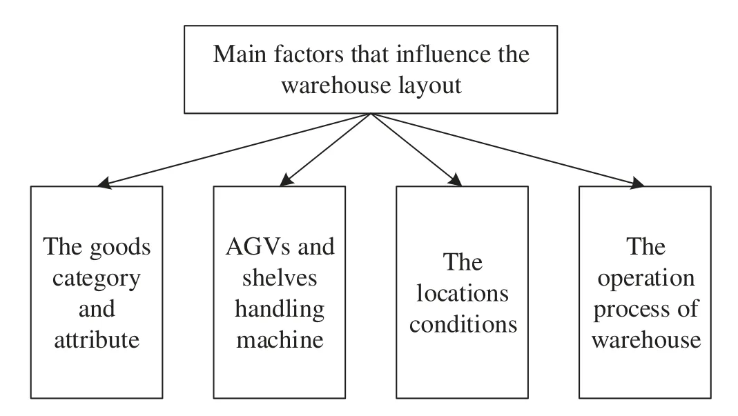
Figure 3:Factors that influence the automated warehouse layout

4.1.1 Paths Arrangement

There are three popular patterns for paths arrangement as shown in Fig.4[27,28]:(a)single oneway route pattern;(b)single two-way route pattern;(c)double one-way route pattern.

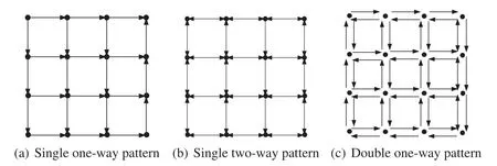
Figure 4:Common paths arrangement patterns

In the single one-way pattern,AGVs travel along with the exact directions,so the probability of collisions can be decreased significantly.However,it may reduce throughput because AGVs could not travel backward.

In the single two-way pattern,the flexibility of systems is improved since the map is bi-directional.However,the route planning becomes complicated because there may exist more types of collisions(e.g.,head-on and cross-road collisions),and thus the probability of collisions is increased.

The double one-way pattern is the combination of the above two patterns.It brings benefits in regard of both systems’flexibility and route-planning complicity.However,it needs more space to arrange workstations.Therefore,it is suitable for super-large-scale environments.

4.1.2 Facilities Arrangement

There are four popular warehouse layouts,as shown in Fig.5[29,30].

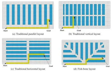
Figure 5:Common warehouse layouts

Figs.5a–5c are three common environments,where shelves are arranged according to the rules of rows and columns,and there is a channel beside them for accesses;Fig.5d is a recently developed map due to the rapid development of automated warehouses,and it looks like fish bones.In fish-bone environments,shelves are arranged on both sides of the diagonal.Theoretically,it can increase the storage of goods,but it is inconvenient for AGV access and may lead to a system deadlock because signals may be blocked.

4.1.3 Storage Environments Modeling Methods

The objective of environment modeling is to arrange many workstations and paths in limited areas and present them using mathematics language,and several modeling methods are as follows:

(a)Topological Map Method

The topological map method belongs to graph theory [31],as shown in Fig.6,where nodes indicate workstations with specific significance,e.g.,paths intersections,AGVs parking areas,and AGVs charging locations,etc.The arcs connected between related nodes indicate AGVs’paths.

A topological map is a high abstraction of natural environments.Instead of measuring the sizes of AGVs or obstacles,we can pay more attention to route-planning strategies.

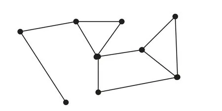
Figure 6:Example of the topological method

However,the accuracy is not very satisfying since it neglects the sizes of objects.

(b)Free Space Method

The free-space method operates “bloating” based on the max diameters of obstacles [32].It considers the obstacles as convex polygons,and divides the environment into obstacles areas (i.e.,the grey areas),the obstacles-free regions,and the solid lines indicate AGVs’paths,as shown in Fig.7.

Figure 7:Example of free space method

However,the disadvantage of the method is it may not work well in environments with many obstacles.

(c)Grid Method

The grid method is one of the prevalent environment modeling methods,which has been widely used in mobile robot route planning.The natural environments are abstracted using rasterizing,as shown in Fig.8.The environment is divided into small grids,and every grid connects others without overlaps[33–35].

The grid map can be classified into the following categories:(a)free grid map,where no obstacles are inside the map;(b)obstacle grid map,where the grid is wholly or partly filled by some obstacles.Every grid denotes a workstation,where the grey grids denote obstacles and the numbers in grids denote the coordinates.

Figure 8:Map of the grid method

4.1.4 Storage Environments Rasterization and Establishment

In anm×nwarehouse,the coordinates of the upper-left corner are(x=0,y=0),the lower-right corner is(x=n-1,y=m-1),as shown in Fig.9[17].Given the length(or width)of AGVs isLAGV;the length(or width)of each grid isLgrid=LAGV+δ(δis a positive number,which indicates the safety margin for AGVs);the length of the storage environment isLenvand the width isWenv,so the number of grids in columns isRgrid=and the number of grids in rows isCgrid=where[·]means down-rounding.Then,the storage environments are divided inton=[Rgrid×Cgrid]′grids,where [·]′means up-rounding.

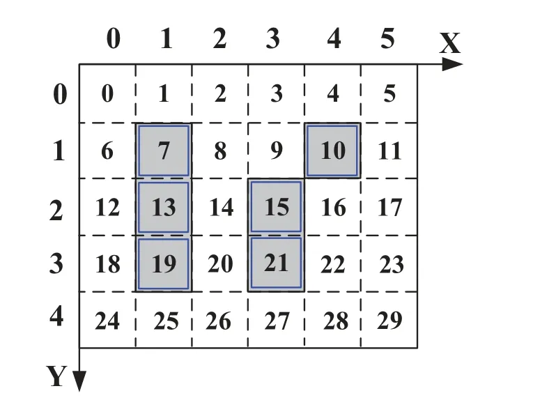
Figure 9:Example of rasterizing storage environments

According to the above rasterizing method,the warehouse environments are designed and planned usingOpenCV-Pythonas follows [36]: (a) taking a picture of the vacant ground and converting it into a standard quadrilateral using Field-Programmable Gate Array (FPGA) [37] and perspective transformation [38,39];(b) drawing the approximate storage area boundary on the above standard rectangular image,i.e.,extracting the storage area using the background filtering and the foreground extraction[40,41];(c)computing the external enclosing rectangle to obtain the exact area boundary[42];(d)completing grids division of the storage area,i.e.,computing the number of workstations in rows and columns;(e) finishing the environment layout,i.e.,reviewing whether the planning results are consistent with the requirements.Since the optimal storage environment layout can be obtained automatically,it significantly reduces the labor force and the energy cost.

4.2 Operation Optimization in Automated Warehouses

4.2.1 Materials Flow in Warehouse

The materials flow consists of the following parts:(a)receiving,i.e.,picking up shelves from input locations and transporting them to designated locations;(b)delivering,i.e.,picking up shelves from designated locations and transporting them to output locations.

Most of the existing publications conducted shelves-picking decisions sequentially,so the time delay of the previous step may affect the next operations[43].Xie et al.[44] proposed an integrated shelves-picking procedure by integrating receiving and delivering operations to reduce the influence of delays,and they adopted the conventional task-split following[45]into receiving operations.Moreover,de Koster et al.[26,46]divided the storage area into multiple zones by combining the idea of task-split and zone-control.However,the task splitting may generate additional waiting time because AGVs should visit many stations to collect all parts of the order.

4.2.2 AGVs Fleet Size

Overestimating AGVs fleet size could lead to high cost and frequent congestion,while underestimating may not ensure the completion of tasks[47].The methods of estimating the optimal AGVs fleet size can be categorized as follows: (a) simulation-based methods;(b) analysis-based methods.To the best of our knowledge,Muller et al.[48] is the first focused on analysis-based methods,he determined the optimal number of AGVs by approximately calculating the total travel time,and they showed that with the increase of the number of AGVs,the average operation time decreases and the average throughput volume increases.Moreover,Ji et al.[49] developed an approximately analysisbased method to estimate the number of AGVs when the total number of idle AGVs is stable.Newton[50]is the first proposed simulation-based method to estimate the minimum of AGVs fleet size,and then Kasilingam et al.[51]developed the model of the method.Although the analysis-based methods may underestimate AGVs’fleet size compared to simulation-based methods[52],the simulation-based methods are time-required techniques.

4.2.3 Electrical Energy Management

Although the electrical energy management is essential,it is often neglected in publications.A new energy supply way(i.e.,Inductive Power Transfer System(IPTS))is developed currently to replace the traditional way of using batteries,but nearly 8%of the European producers employed IPTS in 2006,and the energy supply using batteries is the most widely used manner[53].

The factors that affect battery management are as follows [54]: (1) the number of charging positions in charging stations;(2) the working time of AGVs before the electric energy level is low.Berenz et al.[55] developed the method of evaluating the risk of battery depletion for AGVs using probability density functions.Kabir et al.[56] developed a method to achieve more running time for AGVs using Targeted State of Charge(TSC),and they showed that the charging time for AGVs could be obtained using optimization,e.g.,Petri Net,and applied it in environments such as container terminals and hospitals.

4.2.4 Storage Allocation Policies

(a)Random-Storage Allocation

The random-storage allocation refers to assigning shelves to empty locations with equal probability(e.g.,the same travel distance or the same travel time)[57].

However,the policy may lead to low space utilization and increase AGVs travel distances.

(b)Cheapest-Storage Allocation

Herein,the“cheapest”refers to the distance(e.g.,Euclidean or Manhattan)being the shortest,or travel time is the least.

Theadvantagesof the policy are as follows[58]:(a)it is easily applied for complex environments;(b)it could perform well if all shelves can be used with the same frequencies.On the other hand,it may lead to imbalance since goods are often stacked around the entrance but emptier gradually towards the back.

(c)Specific-Storage Allocation

It classifies goods into several categories based on their characteristics and stores them in many specific areas,and then it uses a random-storage allocation policy to further choose the storage location in the region[59].Cruz-DomAnguez et al.[60]employed two-level neural networks in storage allocation,the first level has one neuron,which receives input information and dispatches goods specific channels;the second level has eight neurons,which arrange goods to designated areas.

The objective of the specific-storage allocation is to satisfy the low-storage space requirements,and itsadvantagesare as follows [61]: (a) it can shorten decision-making time if servers are familiar with the layouts;(b)it is suitable for scenarios that goods have different weights and sizes.On the other hand,the space utilization is not high because some locations are reserved only for certain goods.

(d)Full-Turnover-Storage Allocation

The main mechanic of the policy is the Cube-per-Order Rate(COR),i.e.,the ratio of total required space and number of AGVs travels.

Therefore,the goods with higher CORs are located at the most accessible locations,and those with lower CORs are located towards the back of the warehouses[54].Moreover,the turnover rates can change constantly and it may lead to goods overstocks.

(e)Similar-Storage Allocation

The goods allocation belongs to goods clustering problems,which can be solved using median methods.For example,when an AGV needs to pick up two similar goods,it can save more energy if they are closer to each other.

However,most publications fail to notice the possible relationship among goods.

5 Automated Guided Vehicles Scheduling in Warehouses

AGVs can become idle when they finish their current tasks,and the goal nodes of previous tasks are often not the start nodes of the following tasks.Common principles of AGVs scheduling are as follows [62,63]: (a) minimizing AGVs’travel distances;(b) minimizing AGVs’waiting time;(c)minimizing number of AGVs;(d)minimizing warehouses’operation cost.

The scheduling method in warehouses includes: (a) offline AGVs scheduling;(b) online AGVs scheduling,and the methods can be classified into the following categories[64]:(a)First-Come-First-Served (FCFS),which is one of the most widely used methods,and the operation orders entirely depend on the issued time of tasks;(b) greedy method,which is used to minimize operation cost;(c) task priority-based method,the objective of the method is to deliver emergent goods (e.g.,fresh foods)to customers as soon as possible.

5.1 Classical AGVs Scheduling Methods

The process of AGVs schedule is as follows[26]:(a)when a task is issued,the start/goal nodes and the expected delivery time are sent to the scheduler at the same time;(b) all possible combinations between AGVs and tasks are generated in scheduler;(c) the distances between AGVs and tasks are computed,an idle AGV with the minimum travel time is selected as the optimal AGV;(d) the computation results are dispatched to the selected AGV.The lifecycle of a delivery task is shown in Table 1.

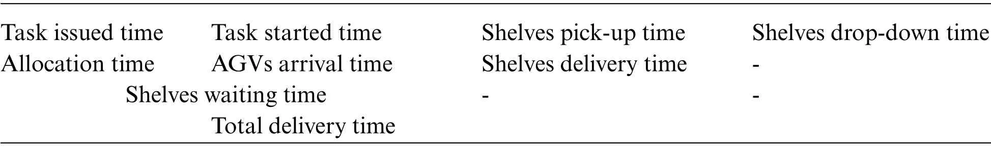
Table 1:The lifecycle of a delivery task

In general,AGVs scheduling could be categorized as Single-Task Allocation (STA) and Multi-Task Allocation (MTA) [65]: an AGV conducts one task once in STA,which is a commonly used method;MTA refers to assigning multiple tasks to an AGV.However,there are few publications related to MTA even though it can increase the efficiency of systems[66].

Yalcin et al.[67] focused on Puzzle-Based Storage (PBS) scenarios with the minimum number of moves: first,they transformed the problem into a state-space problem;then,they employed the A* algorithm to find an optimal AGV for new issued tasks.Moreover,they presented three estimating functions to estimate the upper bound of escorts’number in each episode.However,the conventional methods assign tasks only based on the distances between AGV and tasks,which may lead to a local minimum,and traffic congestion may have a significant influence on the performance.Fazlollahtabar et al.[68,69] developed a mathematical model and proposed a heuristic solution by considering the traffic congestions,and they showed that AGVs scheduling and route planning could be combined,but most publications only focused on one of them.

In our opinion,the RL algorithms used in the existing publications can allow AGVs to have learning capabilities (i.e.,decide which actions to take at the moment),but the AGVs’scheduling problem in dynamic or stochastic environments is barely tackled.

5.2 AGVs Scheduling in Chessboard-Like Warehouses

The classical AGVs scheduling methods are not suitable for current environments with many nodes.They failed to notice the problem of energy cost and indicate the characteristics of chessboardlike warehouses,i.e.,AGVs can only travel in the cardinal directions and turn at nodes[70].

Most publications used Euclidean distance,i.e.,k-Nearest Neighbor(k-NN),to evaluate distance,but the disadvantages of it are as follows:(a)it may not work well when data samples are imbalanced;(b)the computation amount is large for large-scale environments,so it requires data pre-processing;(c) the shortest Euclidean distance does not mean the shortest AGVs traveling distance in grid environments.Therefore,Euclidean distance-based scheduling method is not suitable for chessboardlike warehouses[71].

Manhattan distance represents the sum of the projection lengths of lines between two nodes,i.e.,Dm(i,j)=which indicates the Manhattan distance betweenPi(xi,yi)andPj(xj,yj).Although the computation amount is decreased significantly in grid environments,it does not consider the turns,so the scheduling results may not be the least energy-cost[70].The Dijkstra’s algorithm is a classical routing algorithm based on graph theory,and we can integrate the AGVs route planning into AGVs scheduling,i.e.,the present Dijkstra’s algorithm-based scheduling algorithm.The Dijkstra’s algorithm-based AGVs scheduling algorithm computes the optimal solution using Breadth-First Search(BFS),so that we can obtain not only the location of the optimal agent but also the timeshortest route [72].Although Dijkstra’s algorithm-based AGVs scheduling algorithm is superior to other algorithms in chessboard-like environments,there are few publications related to chessboardlike warehouses[70]and this research area needs to be further investigated.

6 Automated Guided Vehicles Route Planning in Warehouses

AGVs route planning belongs to the shortest route optimization problem.Common methods include Dijkstra’s algorithm [8],A* algorithm [9],D* algorithm [10,73],Artificial Potential Field(APF) [74],Probabilistic Roadmap (PRM) [75],Rapid Random Tree (RRT) [76],Neural Network[77],Genetic Algorithm [78],Ant Colony Algorithm and other intelligent algorithms [79–81].Their mechanisms and performs are shown in Table 2.However,management is a challenge because collisions and deadlocks may occur in bidirectional environments,moreover,it is essentially different from the route selection problems of graph theory.

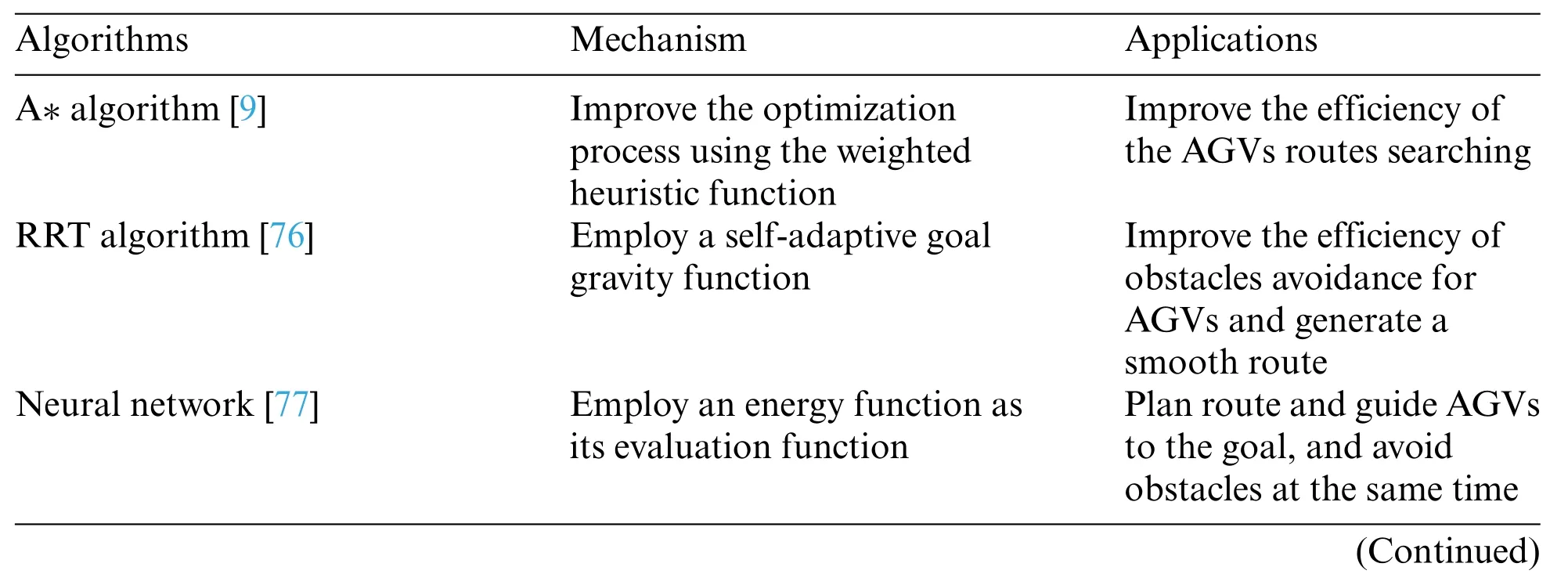
Table 2:Application of intelligent algorithm in AGVs route planning

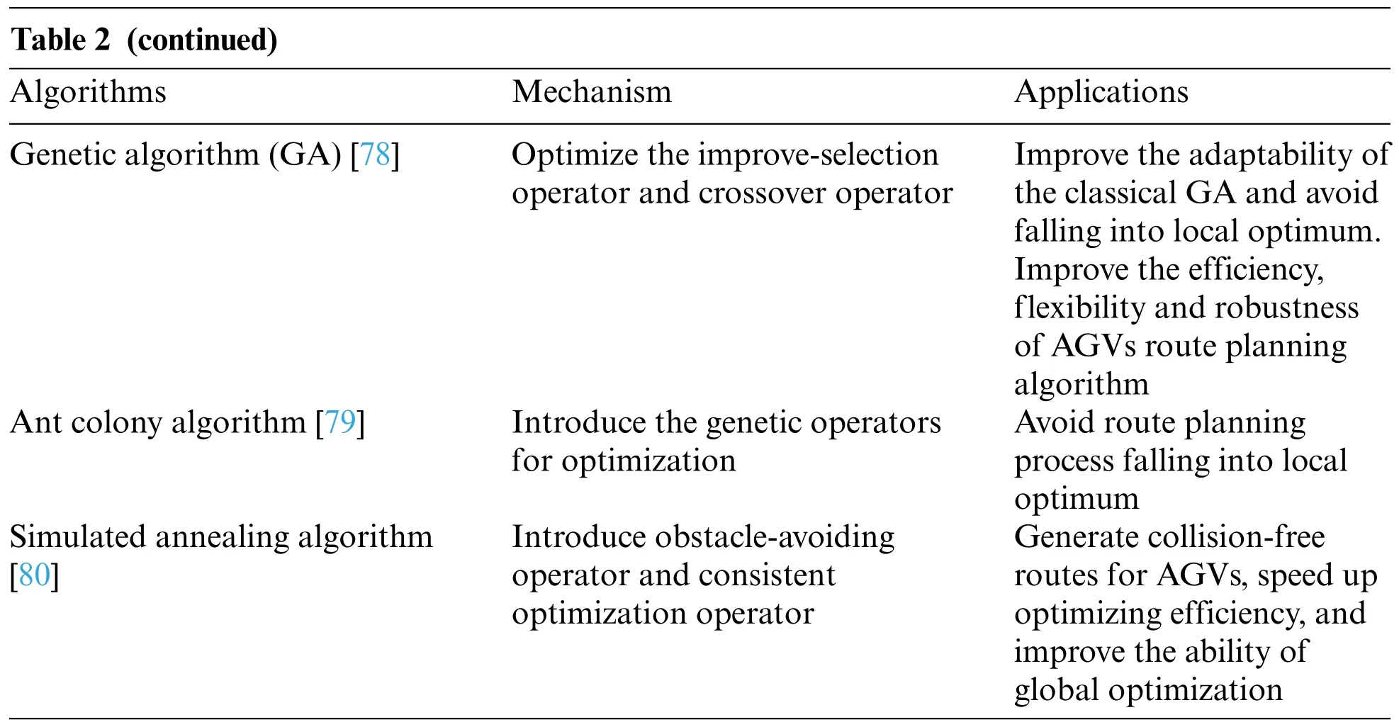
Table 2 (continued)Algorithms Mechanism Applications Improve the adaptability of the classical GA and avoid falling into local optimum.Improve the efficiency,flexibility and robustness of AGVs route planning algorithm Ant colony algorithm[79] Introduce the genetic operators for optimization Genetic algorithm(GA)[78] Optimize the improve-selection operator and crossover operator Avoid route planning process falling into local optimum Simulated annealing algorithm[80]Introduce obstacle-avoiding operator and consistent optimization operator Generate collision-free routes for AGVs,speed up optimizing efficiency,and improve the ability of global optimization

6.1 Single-AGV Route-Planning Methods

6.1.1 Classical Single-AGV Route Planning

The advantages and disadvantages of several commonly used AGVs guidance systems[82,83]are shown in Table 3.

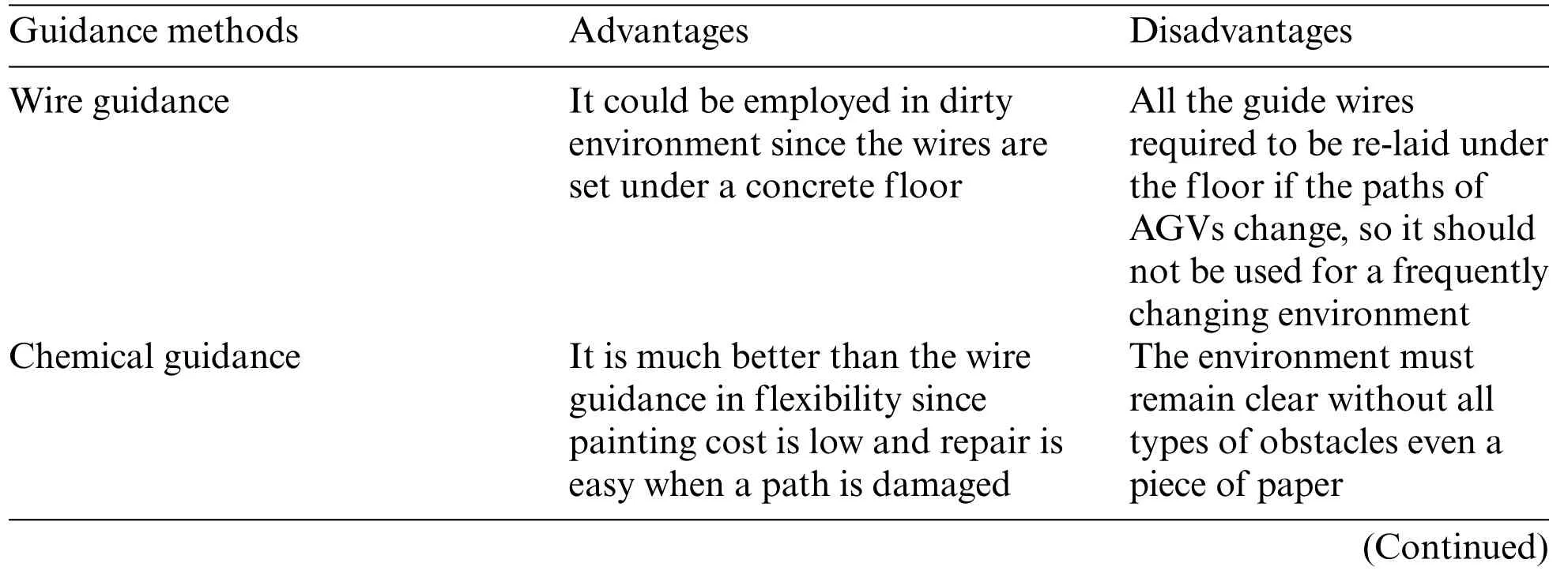
Table 3:Comparison of different type of guidance

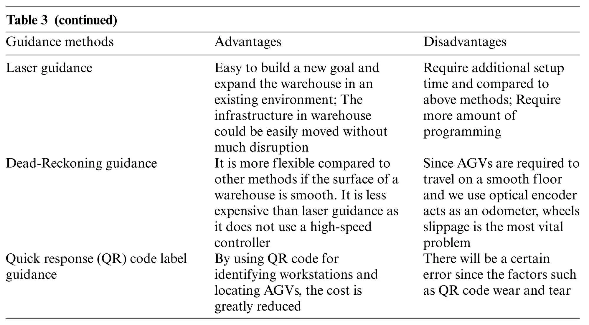
Table 3 (continued)Guidance methods Advantages Disadvantages Laser guidance Easy to build a new goal and expand the warehouse in an existing environment;The infrastructure in warehouse could be easily moved without much disruption Require additional setup time and compared to above methods;Require more amount of programming Dead-Reckoning guidance It is more flexible compared to other methods if the surface of a warehouse is smooth.It is less expensive than laser guidance as it does not use a high-speed controller Since AGVs are required to travel on a smooth floor and we use optical encoder acts as an odometer,wheels slippage is the most vital problem Quick response(QR)code label guidance By using QR code for identifying workstations and locating AGVs,the cost is greatly reduced There will be a certain error since the factors such as QR code wear and tear

Single-AGV route planning can be used both in static and dynamic environments,we can use environments perception and local propagation algorithm in static environments,but it is not a trivial task in dynamic environments because the planned routes may be unavailable at some time[84].

Radio-Frequency Identification (RFID) is one of the common route-planning methods,and warehouses could be extended easily using RFID,but the main disadvantage is that accuracy will reduce with the increase of speed under the same weights of shelves[85],as shown in Table 4.Since the sampling frequency is fixed,when AGVs travel faster,the time delay can be more apparent,so we should reduce the speed of AGVs while turning.We can fix a camera at the overhead corner to obtain the locations of AGVs usingOpenCV(refer to Section 4),and we can determine their next move using Robot Operating System(ROS),as shown in Fig.10[86].

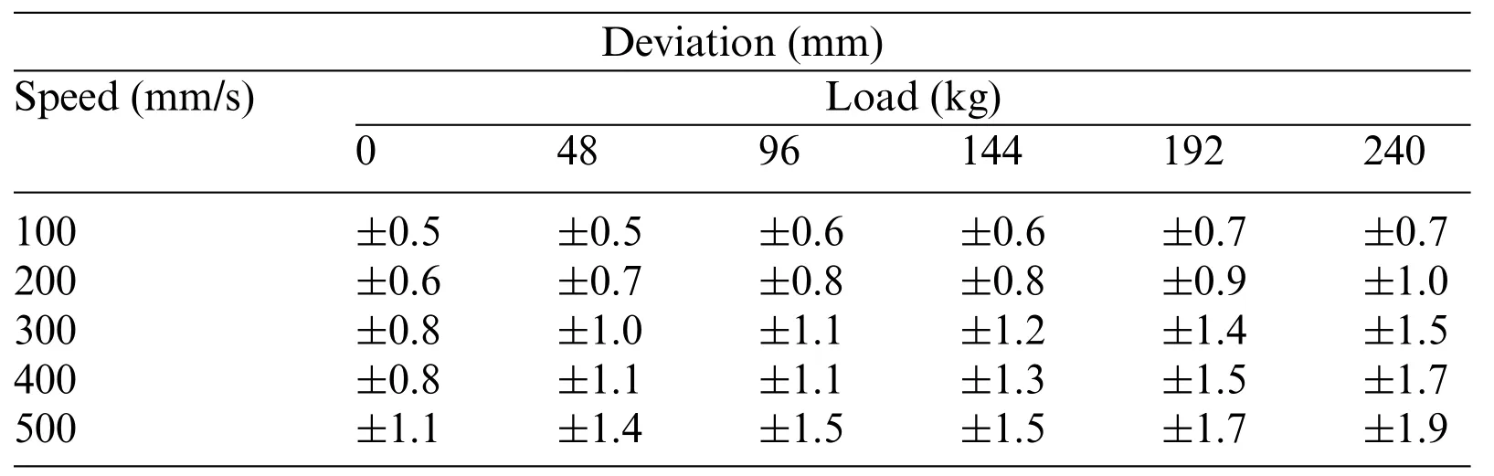
Table 4:The navigation performance test under different shelves conditions

Since the structure of the Dijkstra’s algorithm is simple,it had been used to perfectly solve the route-planning problem in a small-scale environment[8,72,87–89].Ogata[90]compared the Dijkstra’s algorithm,the A* algorithm,and the LPA* algorithm (i.e.,improved version of the A* algorithm).Since the A*algorithm(or the LPA*algorithm)contains heuristic mechanisms[91],it is more efficient than the Dijkstra’s algorithm in large environments.However,the planned routes may not be optimal sometimes.Moreover,Wu et al.[92,93] presented Colored Resource-Oriented Petri Net (CROPN)models,which can be employed to solve AGVs route-planning problems in environments with a few nodes.Lim et al.[81]divide the free-range environments into many grids to solve the route planning for Unmanned Aerial Vehicles(UAVs).

Figure 10:The mechanical design of visual navigation

For simplicity,as shown in Fig.11,the process of generating equidistant shortest routes from node 1 to node 15 is shown in Table 5.

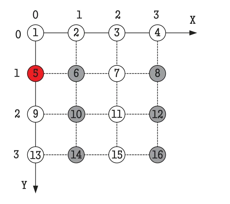
Figure 11:Simplified rasterized warehouse environment

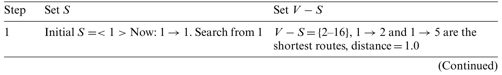
Table 5:The process of generating equidistant shortest routes

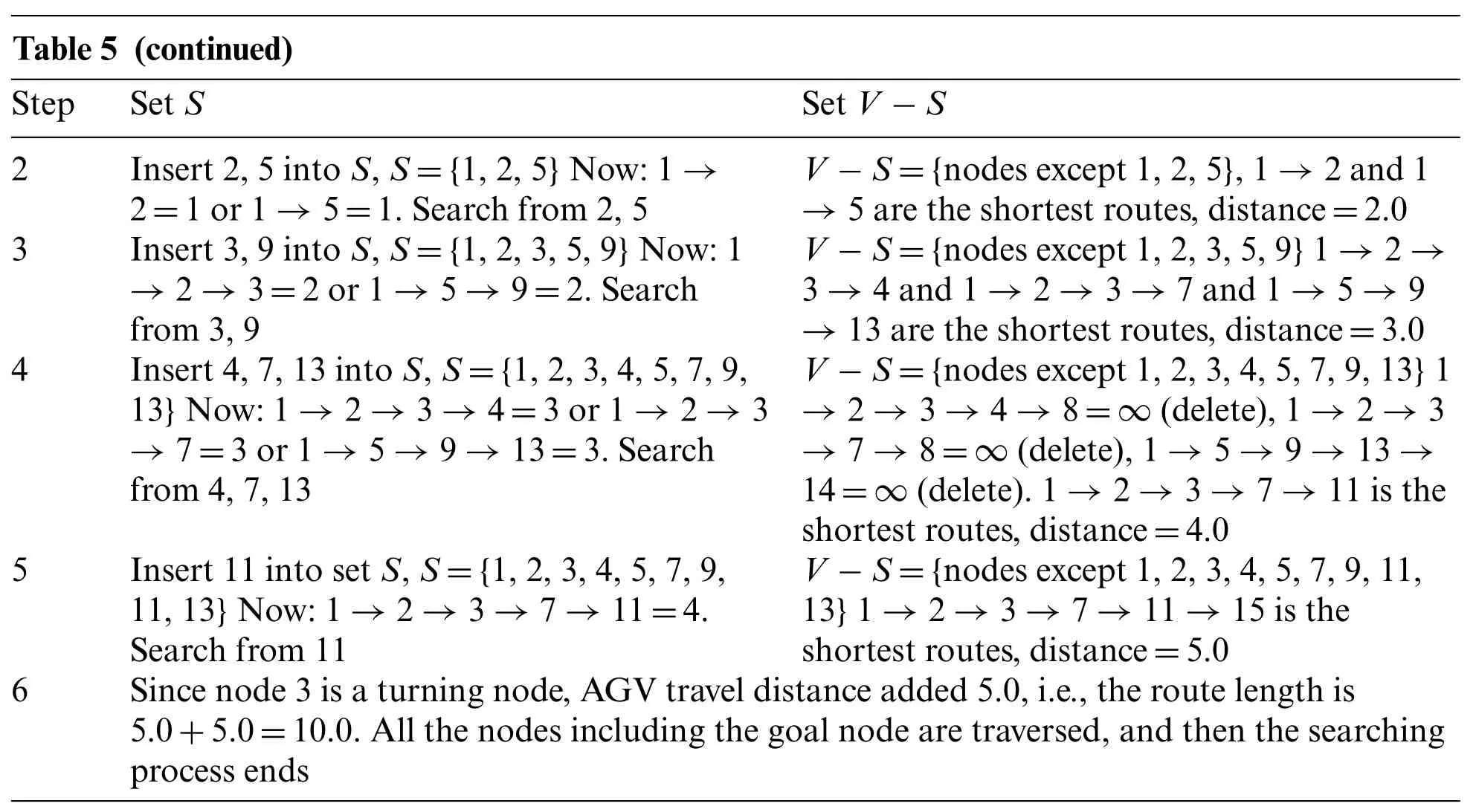
Table 5 (continued)Step Set S Set V -S 2 Insert 2,5 into S,S={1,2,5}Now:1→2=1 or 1→5=1.Search from 2,5 3 Insert 3,9 into S,S={1,2,3,5,9}Now:1→2→3=2 or 1→5→9=2.Search from 3,9 V -S={nodes except 1,2,5},1→2 and 1→5 are the shortest routes,distance=2.0 V -S={nodes except 1,2,3,5,9}1→2→3→4 and 1→2→3→7 and 1→5→9→13 are the shortest routes,distance=3.0 4 Insert 4,7,13 into S,S={1,2,3,4,5,7,9,13}Now:1→2→3→4=3 or 1→2→3→7=3 or 1→5→9→13=3.Search from 4,7,13 V -S={nodes except 1,2,3,4,5,7,9,13}1→2→3→4→8=∞(delete),1→2→3→7→8=∞(delete),1→5→9→13→14=∞(delete).1→2→3→7→11 is the shortest routes,distance=4.0 V -S={nodes except 1,2,3,4,5,7,9,11,13}1→2→3→7→11→15 is the shortest routes,distance=5.0 6 Since node 3 is a turning node,AGV travel distance added 5.0,i.e.,the route length is 5.0+5.0=10.0.All the nodes including the goal node are traversed,and then the searching process ends 5 Insert 11 into set S,S={1,2,3,4,5,7,9,11,13}Now:1→2→3→7→11=4.Search from 11

However,the above publications failed to verify the route-planning efficiency of the algorithm in environments with many nodes.Them×nautomated warehouses focused in this paper are as shown in Fig.12a–12c,wheremandnrepresent the number of rows and columns of the environments,respectively.The grey grids indicate obstacles,white grids indicate the channels for AGVs,and numbers in grids indicate the number of nodes(i.e.,the number of nodes starting from(x=0,y=0)and marked as 1,2,3...n).Red,green,and blue solid squares indicate the start nodes of AGVs,and solid circles indicate their goal nodes[94].

6.1.2 The Shortest Length-Time Dijkstra’s Algorithm-Based Single-AGV Route-Planning Methods

As shown in Fig.12,the route-planning environments are more complex because more than one equidistant shortest route can exist between two nodes.However,the classical Dijkstra’s algorithm can only find one shortest route and skip over other routes with the same distance.

In our previous work,we improved the classical Dijkstra’s algorithm by considering turns of AGVs to find the optimal routes with both the shortest distance and travel time[72].The improved Dijkstra’s algorithm reserved all nodes with the same lengths to the source as the intermediate nodes,then searched again from all intermediate nodes until to the goal node.Through multiple iterations,all the shortest routes with the same distance can be found.Moreover,we considered whether a node is a turn or not based on Eq.(1)to reduce the number of turns in the route to improve the efficiency of warehouses.

where(Xm,Ym)denotes the coordinates of current nodes;(Xm+1,Ym+1)the next nodes;(Xm-1,Ym-1)the previous nodes.

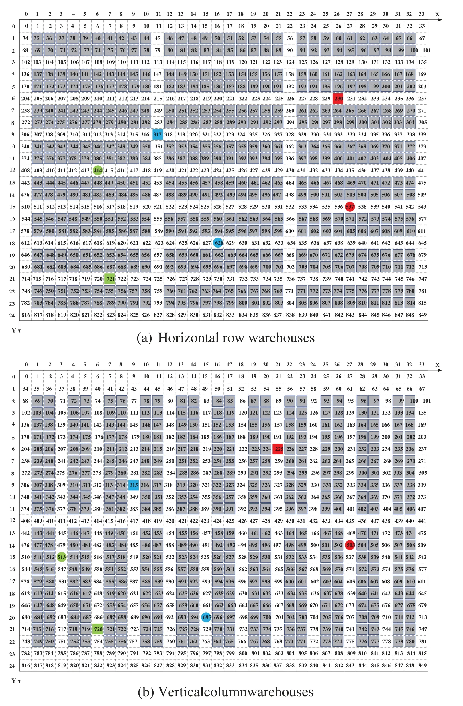
Figure 12:(Continued)

Figure 12:Common paths arrangement patterns

6.1.3 AI-Based Decision-Making Algorithms

The AI-based algorithms are introduced in route planning due to the abilities of thinking,reasoning,and memory,and they can be categorized as follows[95]:(a)knowledge-based algorithm;(b) heuristic algorithm;(c) approximate logic algorithm;(d) cognitive algorithm.The comparisons of the above algorithms in real-world scenarios are shown in Table 6 [96],where the evaluation was indicated with a number scale.

Table 6:The comparisons of AI-based methods adaptability to real-world applications

Table 6 (continued)Methods Evaluation criteria Multi-objective Traffic rules Environment evolution Real-time Stability Leeway Human-like Risk -1 2 2 2 1 -1 Task 1 1 1 1 2 -1 Game 3 2 2 1 2 1

(a)Human-like decision-making algorithms

The learning steps of humans are shown in Table 7[95].

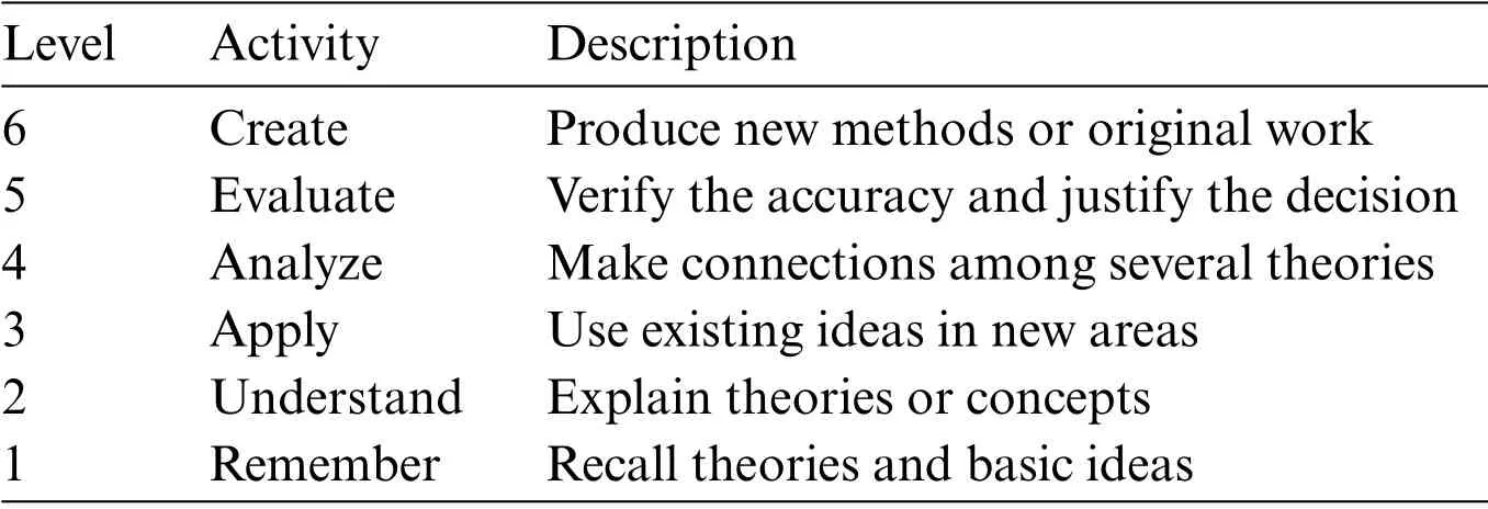
Table 7:Bloom’s taxonomy of human learning

The 1stlevel is the traditional ability that both humans and computers can have,and no AI is required;the 2ndlevel refers to extend theories based on current situations;the 3rdlevel refers to applying AI to test,describe or validate new input data;the 4thlevel refers to predict,compare and analyze relationships among different elements;the 5thlevel can be used to make a trade-off in complex systems;the 6thlevel refers to create new methods,which is the highest level of the human learning.

From our perspective,AI can assist humans for the first three levels and replace humans in the 5thand 6thlevels,the successful cases(e.g.,parameter setting networks)indicates the possibility of creating.

(b)Heuristic algorithms

The heuristic algorithms were inspired by the natural evolution process,many effective learning methods(e.g.,Support Vector Machines(SVM)and Evolutionary Algorithm(EA))can be employed,and the most common heuristic algorithm for AGVs route planning is the A*algorithm[97].

Theadvantagesof heuristic algorithms are as follows: (a) reducing computation complexity in small environments;(b) running faster than exhaustive methods.However,it uses the current state rather than the global state,so that it could lead to a locally optimal solution.

(c)Approximate reasoning algorithms

The approximate reasoning algorithms contained multi-valued logic,so the solutions have approximation dimensions.Recently,Artificial Neurons Networks(ANNs)have contributed an alternative method for approximating,and the approximate reasoning algorithm is close to the human reasoning process.

Theadvantageof approximate reasoning algorithms is they are fuzzy-based methods,so the demand for accuracy is not strict.On the other hand,the challenging problem is to ensure learning correctly[98],so some labeled data is needed to increase the accuracy.

(d)Knowledge-based inference engines

The knowledge-based inference engines rely on deductive reasoning mechanisms,and the most popular algorithm is the rules-based reasoning algorithm (e.g.,Expert System (ES)) [99].Another common model is Finite State Machine (FSM),i.e.,the systems are described using several states and transitions among them,and both the ES and the FSM are triggered by environmental changes.Moreover,warehouses could be extended to dynamic Bayesian networks with Markov properties[100,101].

Theadvantageof knowledge-based inference engines is they are robust in any unexpected situations.On the other hand,they are prior knowledge required methods.

6.1.4 AI-based Single-AGV Route-Planning Algorithms

(a)Artificial Neural Networks

Due to the merit of nonlinear functional approximation,Artificial Neural Networks (ANNs)[102,103]are commonly used in route planning[104],and the process is as follows:(a)choosing the maximum incentive from receiving domain like the main input stimulus;(b)choosing a neuron with the maximum incentive as the next neuron if there is a path to the target neuron;(c)repeating above steps,the routes from the start nodes to the goal nodes are obtained.

The common ANNs are as follows [105,106]: (a) multi-layer Forward Networks,which can be used in any unknown environments [107];(b) Hopfield Neural Networks (HNNs) [108];(c) Fuzzy Neural Networks (FNNs);(d) Radial Basis Function Neural Networks (RBFNNs);(e) Adaptive Resonance Theory Neural Networks(ARTNNs)[109],which belong to competitive neural networks.Since ARTNNs do not forget the old knowledge while learning new knowledge,they can avoid local minimum;(f) Self-Organizing Map Neural Networks (SOMNNs) [110],which also belong to competitive neural networks.Since the optimization process can run automatically,they have some similarities with the human brain;

Theadvantagesof ANNs are as follows[111]:(a)they have strong robustness and fault tolerance,and information is stored in distributed ways;(b)they are easy for parallel processing;(c)they can be employed in uncertain systems because they can approximate any nonlinear function;(d) they have strong ability of information processing,and they can deal with both quantitative and qualitative problems.On the other hand,the convergence time of ANNs is long for large-scale environments,so there are no applications in real-world warehouses.

(b)Markov Decision Process

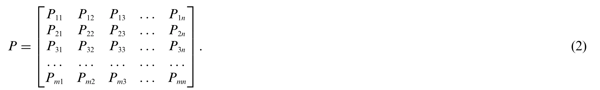
Markov Decision Process(MDP)is a fundamental theory of Reinforcement Learning(RL)[112–115].MDP can be described as a quintuple(i.e.,〈S,A,P,R,γ〉),whereSindicates the finite states set,Athe actions set,andPthe state transition probability matrix[116].Based on the outputs ofPandR,MDP can be classified as deterministic MDP and stochastic MDP,where the outputs are fixed in deterministic MDP,but they are certain distributions in stochastic MDP.Given the probability for entering any adjacent node of AGVs inm×nwarehouses arePij,whereiindicates the current state of the AGV(i.e.,St),jindicates its next state(i.e.,St+1),andPmatrix can be described as follows[17]:

The objective of the MDP method is to find a policy to minimize cost function (e.g.,time or energy)and maximize positive function(e.g.,routes reward or efficiency).

(c)Q-Learning Algorithm

(i)The Classical Q-Learning Algorithm

The supervised learning algorithms are commonly used in route planning,but they are often nonrobust to even small environmental changes [117].The Q-learning algorithm belongs to model-free RL [118–120],which can be considered as asynchronous Dynamic Programming.The Q-learning algorithm relies on rewards and punishments,rather than prior training instances.The learning process of the Q-learning is similar to the classical Temporal Differences(TD)[121],i.e.,agents choose proper actions as the next moves to maximize accumulated rewards [122–124].The pseudo-code of the Qlearning algorithm[125,126]is shown in Algorithm 1.

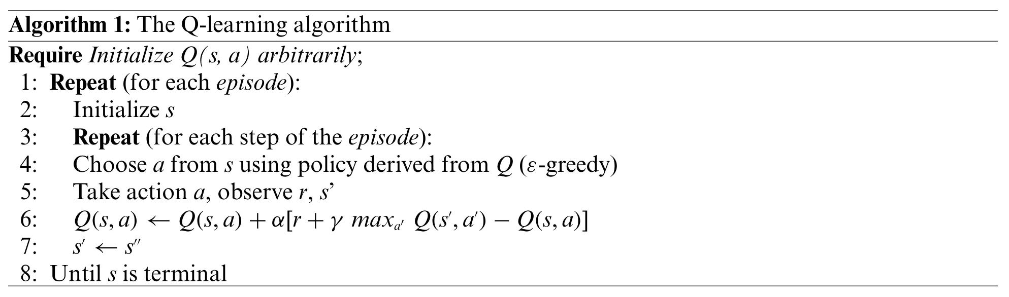
Algorithm 1:The Q-learning algorithm Require Initialize Q(s,a)arbitrarily;1: Repeat(for each episode):2: Initialize s 3: Repeat(for each step of the episode):4: Choose a from s using policy derived from Q(ε-greedy)5: Take action a,observe r,s’6: Q(s,a)←Q(s,a)+α[r+γ maxa′ Q(s′,a′)-Q(s,a)]7: s′←s′′8: Until s is terminal

Theadvantagesof the Q-learning-based route-planning algorithm are as follows[127]:(a)it can deal with route-planning problems in any dimension;(b) it is a model-free algorithm,and it can be used to find optimal actions with any given MDPs.On the other hand,it requires large computations for convergence and large storage to save all the possible actions[128].

(ii)Some varieties of Q-Learning Algorithm

SARSA (State-Action-Reward-State-Action) algorithm uses the form of Q-table and chooses actions with the larger Q-value in the environment as well,as shown in Algorithm 2.But there are some differences between the Q-learning algorithm and the SARSA algorithm,for one thing,the Qlearning algorithm is an off-policy algorithm,but the SARSA algorithm is an on-policy algorithm;for another,the Q-learning algorithm uses Bellman Equation withmax Qto updateQ(s,a),but the SARSA algorithm updatesQ(s,a)using Bellman Equation withoutmax Q.Therefore,the Q-learning algorithm will always choose the shortest route to the goal no matter how dangerous it is,but the SARSA algorithm is quite conservative[129].

Aleo et al.[130] focused on constrained route-planning problems with end-effect,and they introduced the SARSA algorithm in robot route-planning areas.Although the SARSA algorithm can converge to the optimal solution with finite state space,its efficiency has become a vital issue regarding further development.SARSA(λ)is an improved version of the SARSA algorithm,and it improved the convergence using Eligibility Trace(i.e.,backward propagation).Fu et al.[131]developed a fast SARSA (λ) algorithm based on 2ndorder TD error (i.e.,SOE-SARSA (λ)) to improve the convergence rate.

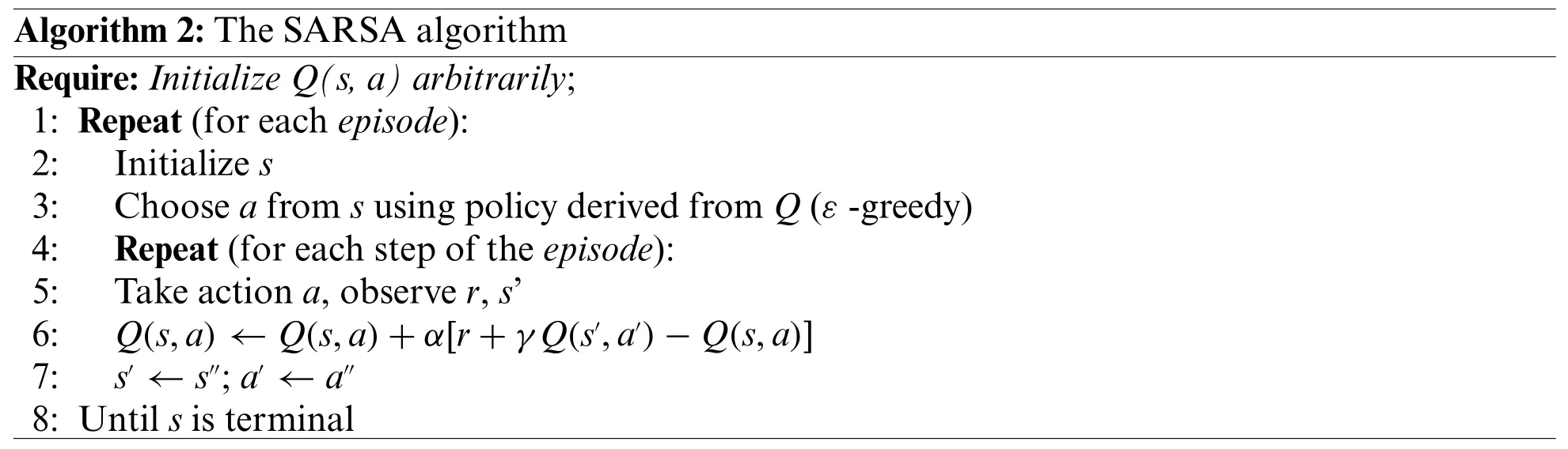
Algorithm 2:The SARSA algorithm Require:Initialize Q(s,a)arbitrarily;1: Repeat(for each episode):2: Initialize s 3: Choose a from s using policy derived from Q(ε-greedy)4: Repeat(for each step of the episode):5: Take action a,observe r,s’6: Q(s,a)←Q(s,a)+α[r+γ Q(s′,a′)-Q(s,a)]7: s′←s′′;a′←a′′8: Until s is terminal

Moreover,Adaptive Heuristic Critic(AHC)algorithm is another alternative method,which used critic-learning mechanisms,and Gachet et al.[132] were the first to employ the AHC algorithm in mobile robot control,they used it to determine proper actions.

From our perspective,it can provide AGVs with the ability to choose optimal actions(i.e.,going forward,turning left,turning right,or stopping) by combining the AHC algorithm and the TD algorithm.

(d)ANNs Combined with Q-learning algorithm

Since the learning speed is low only using the ANNs,and it is impossible to learn all the states only using the Q-learning algorithm,we can combine them to overcome the disadvantages of either[133].In general,there are five outputs for AGVs in warehouses,i.e.,travel forward,stop,turn left 90°,turn right 90°and self-rotate 180°[13],Demircan et al.[134]used ANNs to create route-planning controllers and then used Q-learning algorithm to collect training data for ANNs.Zalama et al.[135]developed a control strategy to choose actions,the Q-learning algorithm is used to determine the behavior and compute the travel velocity of AGVs,and ANNs are used to improve learning operation.

Deep Q-Networks(DQN)is generated by combining the ANNs and the Q-learning algorithms.The preliminary studies of employing the DQN in AGVs route planning on square grids world,showed that the DQN can perform robustly on square grids world[133,136,137].

(e)Reducing Iteration Time of Q-Learning Algorithm

Smart automated warehouses are real-time requirement systems,AGVs should respond to tasks as soon as possible,so we need to pay more attention to computing time.No matter Q-learning algorithm,AHC algorithm,or other RL algorithms,they are operated based on Q-table,i.e.,learning from behaviors of agents through trial-and-error to build the optimal Q-table.We can learn from graph theory to decrease the Q-table convergence time.

Since there are many obstacles(i.e.,negative rewards)in warehouses,the iteration for the classical Q-learning algorithm is very time-consuming.On the other hand,the Dijkstra’s algorithm uses an adjacency matrix to describe environments,so it runs faster than the Q-learning algorithm in the presence of obstacles.Inspired by this observation,we can develop a novel method by integrating the Dijkstra’s algorithm and the Q-learning algorithm to reduce the iteration time and improve the efficiency of systems: First,we could combine the adjacency matrix of the Dijkstra’s algorithm and reward matrix of the Q-learning algorithm into a new matrix(i.e.,Adjacency-Reward(A-R)),and use it to describe environments.Moreover,before AGVs travel,we need to iterate the A-R matrix multiple times to obtain the optimal Q-table,and the dimension of the reward matrix and adjacency matrix are bothn2×n2forn×nenvironments and it takes a long time for iterating.We propose a low-dimensional A-R matrix to describe the environment by considering AGVs’start(and goal)nodes.

(f)Dynamic Programming and Monte-Carlo Search Tree Algorithms

(i)Dynamic Programming-Based Route-Planning Algorithm

The computation of value function is a recursive process,and we need to evaluate the rewards of all adjacent states based on the current state,and the state with the largest reward is taken as AGV’s next state.As shown in Fig.12,the method of computing relationship between the current node and all adjacent nodes is[17]:

wherep(st+1|st,at)indicates the probability of transferring to adjacent statest+1based on the current statestby taking actionat;indicates the reward of transferring to statest+1by taking actionat;γthe discount factor,γ∈[0,1];VT(st+1)the value of each state adjacent to statest.

Without considering obstacle nodes in warehouses,the probability is the same for traveling to surrounding nodes,i.e.,p(st+1|st,at)=γ=1.Eq.(3)can be rewritten as[94]:

whereVuT,VdT,VlT,VrTdenote the state value of upper,lower,left,and right adjacent nodes of AGV’s current nodes,respectively.

(ii)Route-Planning Method of Combining Dynamic Programming and Monte-Carlo Search Tree

The Monte-Carlo Search Tree algorithm can be combined with the Dynamic Programming to improve the speed of route planning [94].First,the classical Monte-Carlo Search Tree algorithm is improved by following steps: (1) the “cutting” operations is added into the “searching” process to determine the expanding directions of search trees;(2) the single-step update is employed for establishing search trees to move the“back-propagation”process ahead of the“simulation”process;(3)the evaluation criteria based on“Move value”is proposed to find the time shortest routes.

Then,the idea of the multi-stage optimization of the Dynamic Programming is introduced,the warehouses are divided based on AGVs’start nodes and their goal nodes.The objective is to increase the efficiency of route planning by reducing the range of route searching.

6.2 Multi-AGV Collision-Free Route-Planning Methods

6.2.1 Classical Multi-AGV Route-Planning Methods

Multi-AGV collision-free route planning belongs to the Multi-Agent Path-Finding (MAPF)problem[138–141],and the most popular methods are time window-based methods[21].There was an improved Dijkstra’s algorithm-based multi-AGV self-adaptive collision-free route-planning approach as follows[87]:it planned routes for each task based on the improved Dijkstra’s algorithm[72];then,it detected and classified potential collisions upon the comparison of nodes’coordinates and occupancy time;finally,a self-adaptive strategy is proposed to solve the potential collisions according to the collisions’types.It presented three strategies as follows: (a) one of the AGVs waits for 5 s or slows down before entering the node;(b)the computer modifies the route of one of AGVs;(c)the system reissues the tasks.

Another common multi-AGV route-planning method is zone-based strategy,i.e.,dividing the route-planning area into many non-overlapping zones and only one AGV in a zone at a time.The traditional zone-based strategy belongs to fixed strategies,where AGVs are not allowed to access other areas,but it can’t work well if the loads are imbalanced among different zones.Ho et al.[20]developed a dynamic zone-based strategy,which improved the traditional strategy in the following aspects:(a)it used zone partition design to maintain balance among different zones,where the zone partition was determined by a relationship coefficient;(b) it improved the traditional design using Simulated Annealing.

The multi-AGV systems are timed discrete event systems and Colored Timed Petri Net(CTPN)is an effective method for modeling,Wu et al.[93]developed a deadlock-free modeling method based on CTPN,and they integrated it with colored edges to build digraphs of routes.However,most publications considered route-planning problems as static problems[142,143],they built time windows for dynamic obstacles and then used local route-planning methods to solve collision-free problems.Despite the effectiveness,it may lead to a sub-optimal solution.Phillips et al.[144] developed an algorithm based on contiguous safe intervals,and the process is as follows:(a)graph construction,i.e.,creating timelines for every spatial configuration using predicted obstacle trajectories;(b)graph search,i.e.,operating route planning using A*algorithm.However,the proposed method does not work well in larger environments.However,the proposed method does not work well in larger environments.

Yan et al.[145] presented two types of travel patterns for AGVs to simplify route planning: (a)cross model;(b) local loop model.As shown in Fig.13,the shaded grids represent the locations of shelves and other grids represent channels,the grids marked with dots represent intersections,and the arrows indicate directions of channels.

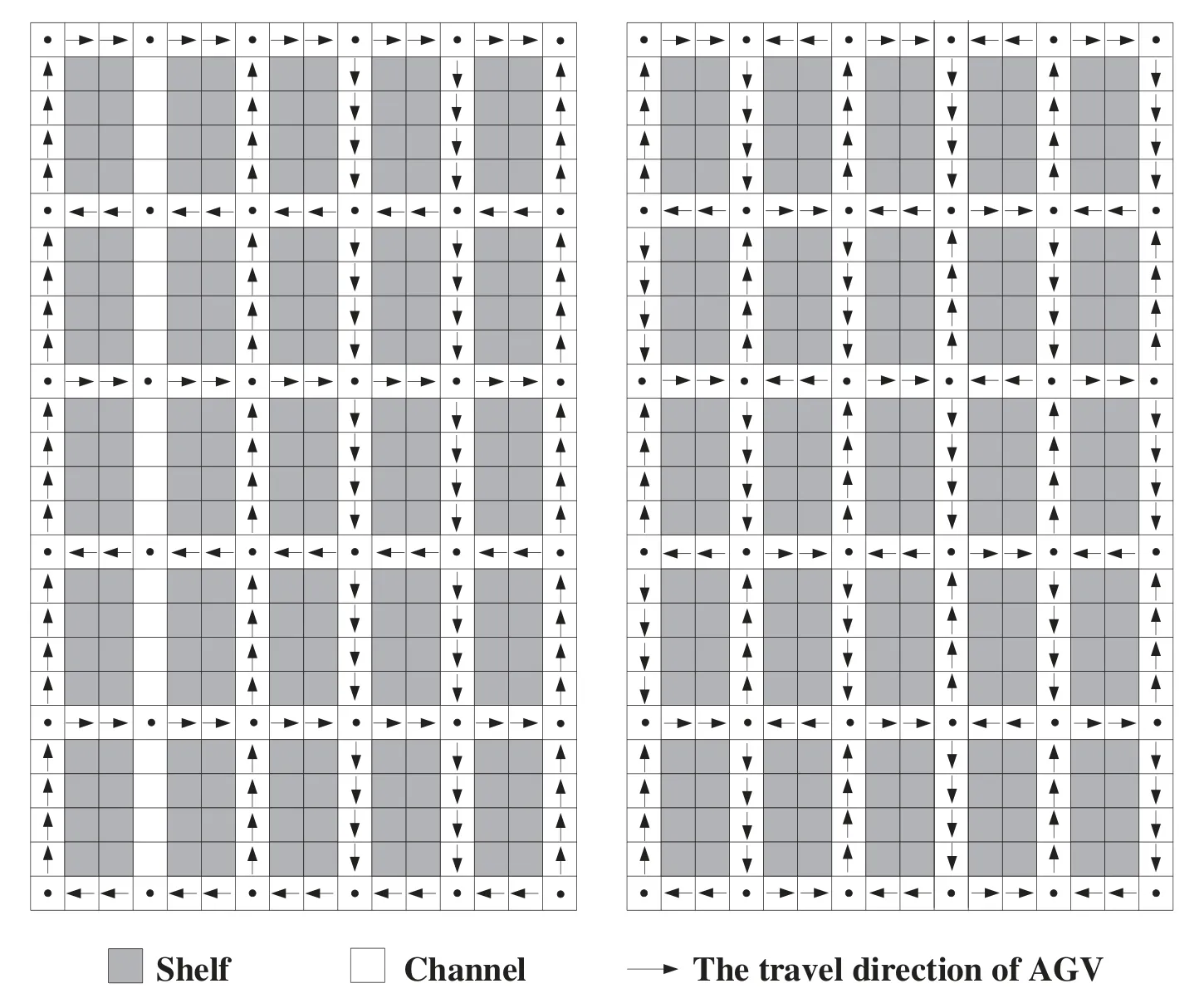
Figure 13:AGVs travel direction patterns

If there are two AGVs in a collision,the most straightforward routes re-planned method is to delete one of AGV’s routes and plan the sub-optimal shortest route for it[146],but it may be difficult for route planning using if-then rules when the number of AGVs becomes large.We can employ the human mind,more specifically,Artificial Intelligence(AI),in route planning to develop the ability of learning.

6.2.2 AI-Based Multi-AGV Route-Planning Algorithms

The state-of-the-art multi-AGV route planning algorithms considered every AGV as an individual with the ability to act autonomously,i.e.,AGVs are equipped with sensors to measure distances to others and detect their positions[147].

Recent work in RL and Deep Reinforcement Learning(DRL)have shown their effectiveness in multi-AGV decision-making problems.Zhang et al.[148]employed the Q-learning algorithm to solve the multi-AGV route-planning problem in urban roads networks scenarios,and they presented that the optimal route may not always be available if an unknown emergency occurs.Panov et al.[133]proposed a multi-AGV fleet coordination algorithm in smart city environments,they combined Convolutional Neural Networks (CNNs) and DRL to make AGVs fulfill tasks in large environments,and they employed the Transfer Learning (TL) to balance multiple objectives.We noticed the paper because the urban scenarios are similar to warehouses.

Similar to single-AGV AI-based route planning,there is also the problem of the “curse of dimensionality”and it needs to reduce state space for route planning.For example,Burkov et al.[149]used the Adaptive Play Q-Learning (APQ) algorithm [150] to restrict the searching space for multi-AGV route planning.

6.2.3 Collisions Resolution Policies Based on Conflicts Classifications

When environments become larger,the number of AGVs and collisions may increase significantly.Despite its effectiveness,the self-adaptive multi-AGV collisions resolution may increase the computation burden of warehouses[87].Therefore,a collision classification-based approach is proposed to improve the real-time performance of systems[88]:First,the collisions in warehouses can be classified into four classifications,as shown in Fig.14.

Figure 14:Common collision classifications

Second,the collision in Fig.14d can be further classified into two types based on whether AGVs are loaded or not.Third,four feasible solutions for the above collisions classifications are presented as follows:(a)selecting the alternative route;(b)waiting for a period before starting to reduce the energy cost of multiple starts and stops;(c)modifying the planned routes;(d)re-dispatching tasks.Fourth,the corresponding solution for each collision classification is selected based on experiments and analyses results.It is worth mentioning that solution(a)and(c)is suitable for collision classification of Fig.14a;solution(b)is suitable for Fig.14b;solution(a)and(c)are both suitable for Fig.14c.

6.2.4 Collisions Resolution Policies Based on Critical Sections

The critical section refers to the parts that contain repeated nodes.This section discusses the location of the collision,and AGVs cannot be regarded as nodes because AGVs should have safety distances to others.

The function of critical sections is to reduce the time wasted finding exact locations of collisions.Manhattan distance indicates the sum of the projection distances of lines formed by two nodes,for example,the Manhattan distance between nodePi(xi,yi)and nodePj(xj,yj)isThe AGV with a smaller Manhattan distance is considered to be modified to minimize the total time of systems,and resolution is as follows[70]:(i)if the goal node of the AGV with a bigger Manhattan distance (i.e.,AGV1) is on the route of the AGV with smaller Manhattan distance (i.e.,AGV2),AGV2should wait forLen×tc+tw(s)before entering the critical sections;(ii)if not,it should wait forLen×tc(s).

Theadvantagesof the critical section-based method compared to the time window-based method[21]are as follows:(1)improves system robustness:it ensures that only one AGV in a certain section avoids collision and ensures the safety margin for AGVs driving;(2) improves the conflict detection efficiency:the coordinates of each of the two nodes and the time of AGVs passing through this node are compared in time window-based method.Although the detection accuracy is improved,the detection efficiency is reduced.In this method,the routes of AGVs are compared in pairs,and if the repeated nodes exist,the length of the critical sections is calculated,otherwise,exiting,so the numbers of comparisons are significantly reduced;(3) reduces computing complexity:it omits the division of conflict types,which improves algorithm’s robustness,reduces the difficulty in applicability,and increases practicability.

7 Conclusion

This paper presented a comprehensive survey on the application of AGVs in warehouses while discussing some key issues,i.e.,AGVs systems,warehouse layout,operation optimization,AGVs scheduling,AGVs routing problem,and AI applications in warehouses.Both centralized and decentralized AGVs systems have their advantages and disadvantages.The warehouse layout and operation optimization(including AGV electrical energy management)play significant roles in building flexible logistic systems.Moreover,AGVs scheduling and route planning are essential for minimizing tasks operation time in current chessboard-like environments.By employing the AI(e.g.,RL algorithms),we can avoid the effectiveness of route-planning algorithms being afflicted by any minor environmental changes.However,the efficiency of RL algorithms can be reduced with the increasing environmental scales.Thus,we proposed an original novel method to accelerate the route-planning efficiency by combining the RL algorithms and Dijkstra’s algorithm.

After reviewing key publications on applications of AGVs in warehouses,we found some problems needed to be further concerned as follows:

· Although the problem of AGVs scheduling has been researched for a long time,the dynamic scheduling methods in chessboard-like warehouses are not adequately attended and discussed.Moreover,integrating idle AGV parking factors into scheduling problems is necessary.

· With the increase of environmental scales,AGVs route planning becomes more complex because the number of nodes is large and routes with the shortest distance may not be the most energy-saving routes.Although the classical AI-based route-planning algorithms (e.g.,the Qlearning algorithm) work well in AGV route planning,they have some limitations (e.g.,the convergence time is large).However,very few publications fundamentally reduce the training time.Therefore,it is an important part of our future work.

· Smart automated warehouses have become more popular.Also,AGVs should be capable of selflearning and self-adaption.Therefore,the flexibility of dealing with environmental changes is more important and few studies have been conducted in this research direction.It is another important part of our future work.

Funding Statement:The authors received no specific funding for this study.

Conflicts of Interest:The authors declare that they have no conflicts of interest to report regarding the present study.