
Comparison of methods for turbulence Doppler frequency shift calculation in Doppler reflectometer
2023-10-08 08:20XiaomingZHONG仲小明XiaolanZOU邹晓岚ChuZHOU周楚AdiLIU刘阿娣GeZHUANG庄革XiFENG冯喜JinZHANG张津JiaxuJI季佳旭HongruiFAN范泓锐ShenLIU刘深ShifanWANG王士凡LiutianGAO高刘天WenxiangSHI史文祥TaoLAN兰涛HongLI李弘JinlinXIE谢锦林WenzheMAO毛文哲ZixiLIU刘子奚and
Plasma Science and Technology 2023年9期
Xiaoming ZHONG(仲小明),Xiaolan ZOU(邹晓岚),Chu ZHOU(周楚),∗,Adi LIU(刘阿娣),Ge ZHUANG(庄革),Xi FENG(冯喜),Jin ZHANG(张津),Jiaxu JI(季佳旭),Hongrui FAN(范泓锐),Shen LIU(刘深),Shifan WANG(王士凡),Liutian GAO(高刘天),Wenxiang SHI(史文祥),Tao LAN(兰涛),Hong LI(李弘),Jinlin XIE(谢锦林),Wenzhe MAO(毛文哲),Zixi LIU(刘子奚) and Wandong LIU(刘万东)
1 School of Nuclear Science and Technology,University of Science and Technology of China,Hefei 230026,People's Republic of China
2 French Alternative Energies and Atomic Energy Commission,Institute for Magnetic Fusion Research,Saint-Paul-Lez-Durance F-13108,France
3 Shenzhen University,Shenzhen 518061,People's Republic of China
Abstract The Doppler reflectometer(DR),a powerful diagnostic for the plasma perpendicular velocity(u⊥)and turbulence measurement,has been widely used in various fusion devices.Many efforts have been put into extracting the Doppler shift from the DR signal.There are several commonly used methods for Doppler shift extraction,such as the phase derivative,the center of gravity,and symmetric fitting(SFIT).However,the strong zero-order reflection component around 0 kHz may interfere with the calculation of the Doppler shift.To avoid the influence of the zerofrequency peak,the asymmetric fitting(AFIT) method was designed to calculate the Doppler shift.Nevertheless,the AFIT method may lead to an unacceptable error when the Doppler shift is relatively small compared to the half width at half maximum(HWHM).Therefore,an improved method,which can remove the zero-frequency peak and fit the remaining Doppler peak with a Gaussian function,is devised to extract the Doppler shift.This method can still work reliably whether the HWHM is larger than the Doppler shift or not.
Keywords: perpendicular velocity measurement,Doppler reflectometer,Doppler shift
1.Introduction
High confinement mode(H-mode),featuring high energy and particle confinement time,has been considered as the baseline operation scenario for the International Tokamak Experimental Reactor project(ITER)[1].The improvement in edge confinement is caused by the edge transport barrier(ETB),which features the reduction in heat and particle transport perpendicular to the magnetic field.The commonly accepted explanation for the ETB is the existence of a strong shear flow caused by the radial electric fieldErin the edge plasma [2].This E×B velocity shear can effectively suppress the edge turbulence [3],which in turn contributes to the formation of the ETB and leads to the L-H transition.Therefore,the measurement ofErwith the high spatial and temporal resolution is crucial to understand the confinement improvement and the transition from L-mode to H-mode in magnetic fusion devices.
The Doppler reflectometer(DR),which can measure the perpendicular velocity,the radial electric field,and the turbulence with high spatial and temporal resolution,has been widely used in various fusion devices,such as EAST [4],HL-2A [5],Tore-Supra [6,7],ASDEX-U [8],DIII-D [9],TJ-II [10],LHD[11],NSTX[12]and so on.The DR launches the probing beam at an oblique angle to the cut-off layer and receives the backscattered signal by the fluctuation structure around the cut-off layer.The movement of the fluctuation structure will bring a Doppler shift into the backscattered signal,and the shifted frequencyfdis 2πfd≃u⊥k⊥[6],whereu⊥andk⊥are the perpendicular velocity and wavenumber of the fluctuations,respectively.Through the measurement of the Doppler shift(fd),the perpendicular velocity can be calculated byu⊥=2πfd/k⊥.In the experiments,the perpendicular velocity is the sum of the E×B velocity to the lab frame and the phase velocity of the density fluctuation:u⊥=uE×B+uphase.With a large torque neutral beam injection heating dominant,theuE×Bis far greater thanuphasein the edge plasma[8,13],which meansu⊥≃uE×B,and thenErcan be evaluated fromEr=u⊥B.In I-mode regime,theu⊥can be converted from positive to negative values due to the alternating transitions between two kinds of turbulence in ion and electron diamagnetic drift directions[14],which may lead to an unacceptable error for commonly used Doppler shift calculation methods.In this paper,the extraction of the Doppler shift foru⊥calculation will be discussed in detail.
There are several methods commonly used for Doppler shift extraction,such as the phase derivative(also called theδ-phase method [15]),the center of gravity(COG),symmetric fitting(SFIT),asymmetric fitting(AFIT)[16],and so on.However,the phase derivative method may cause a large margin of error,which can be used forErfluctuation analysis,but rarely used for the Doppler shift calculation.The COG method requires a high degree of symmetry in the shape of the Doppler spectrogram and is widely used when the spectrum of the DR signal is without a zero-frequency peak.However,in the existence of the zero-frequency peak in the power spectrum,the errors of both the COG and the SFIT may be quite large and unacceptable.Therefore,the AFIT method was used to avoid the interference of the zerofrequency peak to a certain extent.But it has to be mentioned that the AFIT method may lead to an enormous error when the Doppler shift is relatively small compared with the full width at half maxima(HWHM).Here an improved algorithm will be proposed in this paper,which can be used for Doppler shift calculation in most conditions with great accuracy.
The paper is organized as follows.Section 2 introduces the data of DR in the EAST.In section 3,the commonly used methods for estimating Doppler frequency shift are presented,and the improved method for Doppler shift calculation is proposed in section 4.The last part is the conclusion.
2.Data of Doppler reflectometer on EAST
DR,as a powerful diagnostic with a notable spatial and temporal resolution,has been widely engaged in magnetic confinement fusion devices for perpendicular velocity,Er,and turbulence measurements.Since the first DR system was installed on EAST in 2012,several DR systems have been developed on EAST,such as the poloidal correlation DR system [17],the V-band eight-channel Doppler reflectometer [4],and the W-band five-channel DR system [18],and they have become one of the most importantErand turbulence diagnostics on EAST.For the DR,the received signal is obtained from the in-phase(I=Acosφ) and quadrature(Q=Asinφ) of theI/Qmixer,and the complex signal can be written asV=I+iQ=Aeiφ.Here,the phase can be calculated as φ(t)=arctan[Q(t)/I(t)],and signal isBy a sliding fast Fourier transform of the complex amplitude signal,a double-sided power spectrumS(f) can be obtained.The typical double-sided power spectra of DR are shown in figure 1,which can be broadly divided into two categories:one only contains a Doppler shift peak(figure 1(a)),the other contains a Doppler shift peak and a zero-frequency(a peak around 0 kHz,figure 1(b)).Generally,the zero-frequency peak could be caused by the zero-order reflection,which may interfere with the calculation of the Doppler shift [8].
3.Commonly used methods for Doppler shift calculation
Many efforts have been put into the Doppler shift calculation in the past,especially in avoiding the influence of the zero-frequency peak.However,all of the commonly used methods for the Doppler shift calculation have their limitations.Here we will introduce the commonly used methods for Doppler shift calculation and discuss the limitation of these methods in detail.
The phase derivative method can estimate the instantaneous Doppler shift from a phase derivative of the complex signalAeiφ
The phase φ can also be written as: φ=φDoppler+φ0,where the first term is caused by the Doppler shift,and the second term corresponds to the phase modulation due to density oscillation around the cut-off layer[19-21].Owing to the interference of the phase modulation and the zero-frequency peak,the phase deviation method may have a large error in measuring the Doppler shift.However,these interference do not affect the analysis ofErfluctuation,and because of its simplicity,the phase deviation method was almost used forErfluctuation analysis.
The COG method calculates the Doppler shift by taking the weighted spectral mean of a double-sided Doppler spectrumS(f),and the Doppler shift(fd) is derived as
If the spectrum consists of only one Doppler shift peak and the peak is symmetric,the COG method can calculate the Doppler shift accurately.However,when the spectrum contains a zero-frequency peak despite the Doppler shift peak(figure 1(b)) or the spectral wings are asymmetric,the COG method will give an unaccepted error [22].Note that,after filtering out the zero-frequency peak,the COG method is available for the symmetric spectrum with a Doppler peak.
By fitting the double-sided Doppler spectrum with the Gaussian function,the SFIT method can be also used to estimate the Doppler shift,as shown in figure 2.For the spectrum containing only one Doppler shift peak,this method can fit the curve quite well(figure 2(a)),and estimate the Doppler shift with great accuracy.However,when the zerofrequency peak exists,the peak of the fitted Gaussian is between zero and the Doppler shift,which may result in an unacceptable error,as shown in figure 2(b)).
To avoid the influence of the zero-frequency peak,the AFIT method was developed to calculate the Doppler shift frequency,by fitting the asymmetric part of the double-sidedDoppler spectrum with a double Gaussian function[16].Generally,the peak around zero is from the zero-order reflection and is mainly even symmetric,while the Doppler shift peak is asymmetric.So one can remove the zero-frequency peak from the spectrumS(f) by subtractingS(-f)fromS(f):S∗(f)=S(f)-S(-f),as the blue curves in figure 3,and then by fittingS∗(f) with a double Gaussian function the Doppler shift can be calculated.As shown in figure 3,whether the zero-frequency peak exists or not,the double Gaussian(the dash curves in figure 3) can fit the positive peak inS∗(f)(the Doppler shift peak)quite well and calculate the Doppler shift,and the result calculated by AFIT is consistent with the Doppler shift obtained by COG and SFIT after filtering out the zero-frequency peak.Although the power spectrum is asymmetric in the presence of zero-frequency peak,the AFIT method is applicable in figure 3(b).
Because of the advantage of the AFIT method,it has been widely used to calculate the Doppler shift,especially when the zero-frequency peak exists,but it still has its limitations.A simulation of different spectrums was carried out to test the capability of the AFIT method,as shown in figure 4.The Gaussian functionSg=a×e-((f-b)c)2was used to represent the spectrum of DR.Hereais the amplitude,bis the Doppler shift,cis the half width at half maximum(HWHM,γ).In figure 4,the Doppler shift is fixed at 100 kHz(b=100×103),and the HWHM increases from 50 to 200 kHz(c=50×103-200×103).One notes that,although in all the situations the AFIT can fitS∗(f)quite well,the deviation between the peak of the positive part ofS∗(f)andS(f)becomes larger and larger as the HWHM increasing,and the fitted Doppler shift changes from 100.4 to 154.3 kHz while the Doppler shift is fixed at 100 kHz,indicating that the AFIT may bring a large error when the HWHM is relatively large compared to the Doppler shift.
In figure 5,the relative errors of the AFIT method are investigated under different HWHM-Doppler shift ratios(γ/fd).The relative errors will increase quickly when the HWHM is larger than the Doppler shift.In short,the AFITmethod cannot extract the Doppler shift accurately when the Doppler shift is relatively small compared to the HWHM.
4.Improved method to extract Doppler shift
In general,all of the traditional methods used for Doppler shift calculation have their limitations,especially when the zero-frequency peak exists and the Doppler shift is relatively smaller than HWHM.Therefore,an improved Doppler shift calculation method needs to be developed for the complicated experimental data.
In EAST,the DR systems have been widely used for theErand perpendicular velocity measurements and many experimental data in different situations have been obtained,such as the L-H transition,RMP,different auxiliary heating,and so on.To investigate the evolution ofErand perpendicular velocity in these different conditions,a reliable method to calculate the Doppler shift of DR is necessary.However,as mentioned above,all of the traditional methods have their limitations,so a method has been developed for Doppler shift calculation.The core idea is to quickly identify and filter out the zero-frequency peak from the power spectrum and fit the remaining Doppler peak with a Gaussian function.
The algorithm flowchart is shown in figure 6.Firstly,the power spectrum data(S,f)needs to be smoothed to reduce the signal-to-noise ratio.Usually,we used a 4th-order Fourier function(4th-Fourier) to fit the spectrum signal,i.e.whereai,biis the amplitude,ωis the fundamental frequency of the spectrum signal.The fitting function is not exclusive.Therefore,other functions(such as polynomial functions) are also available.The purpose of the fit by the 4th-Fourier is to narrow down the frequency range and obtain a reasonable frequency range of the Doppler peak.
Note that,for the peak with a real nontrivial structure,most current methods for calculating the Doppler shift are not applicable.In this paper,all of Doppler peaks are assumed to be Gaussian functions.Then we can divide the DR power spectrum into four categories,i.e.only a Doppler peak(as shown in figure 7),a Doppler peak plus a highly visible zerofrequency peak(as shown in figure 8),a Doppler peak plus an inconspicuous zero-frequency peak(as shown in figure 9),and a Doppler peak with a poor signal-to-noise ratio(as shown in figure 10).By fitting the smooth spectrum twice times,the existence of a zero-frequency peak can be judged by the number of the local maximum value in the fitted curve.Eventually,a narrower and more reasonable frequency range of the Doppler peak can be obtained.The sample is presented as follows.
For a DR power spectrum with only a distinct Doppler peak(as shown in figure 7),a local maximum value and the HWHM(γ) corresponding to this local maximum value can be obtained in the first 4th-Fourier fit,and this local maximum value frequency is noted asf0(as shown in figure 7(b)).Then,the range fromf0-γtof0+γwas chosen as the frequency range for the second fit(as shown in figure 7(c)).It is distinct that the number of the local maximum value in the second 4th-Fourier fit curve remains 1.Therefore,we finally chose the range fromf0-γtof0+γas the frequency range for the Gaussian fit.
For a DR power spectrum with a Doppler peak plus a highly visible zero-frequency peak(as shown in figure 8),two local maximum values can be obtained in the first 4th-Fourier fit and those frequencies with local maximum values are noted asf1_01,f1_02,as shown in figure 8(b),and theγcorresponds to the HWHM of thef1_02 local maximum value.In addition,a frequency corresponding to the local minimum value exists betweenf1_01 andf1_02,which is recorded asf1_03.After removing the zero-frequency peak,the range fromf1_03 tof1_02 +γwas chosen as the frequency range for the second fit(as shown in figure 8(c)).It is obvious that the number of the local maximum value in the second 4th-Fourier fit curve reduces to 1.Therefore,we finally chose the range fromf1_03 tof1_02 +γas the frequency range for the Gaussian fit.
For a DR spectrum with a Doppler peak plus an inconspicuous zero-frequency peak(as shown in figure 9),only one local maximum value and the HWHM(γ) corresponding to this local maximum value can be gained in the first 4th-Fourier fit,and this local maximum value frequency is noted asf0(as shown in figure 9(b)).Then,the range fromf0-γtof0+γwas chosen as the frequency range for the second fit(as shown in figure 9(c)).In the second 4th-Fourier fit,two local maximum values can be observed,and those frequencies with local maximum values are noted asf2_01,f2_02,as shown in figure 9(b).In addition,a frequency corresponding to the local minimum value exists betweenf2_01 andf2_02,which is recorded asf2_03.It is clear that thef2_01 peak corresponds to the zero-frequency peak.In this case,the inequality(∣f2_02-f2_01∣<min(∣f2_02 ∣,∣f2_01∣)) is false.After removing the zero-frequency peak,the range fromf2_03 tof2_02+γwas chosen as the frequency range for the Gaussian fit,where theγcorresponds to the HWHM of thef2_02 local maximum value.
For a DR spectrum with a poor signal-to-noise ratio Doppler peak(as shown in figure 10),a local maximum value and the HWHM(γ) corresponding to this local maximum value can be obtained in the first 4th-Fourier fit,and this local maximum value frequency is noted asf0(as shown in figure 10(b)).Then,the range fromf0-γtof0+γwas chosen as the frequency range for the second fit(as shown in figure 10(b)).In figure 10(c),two local maximum values can be observed in the second 4th-Fourier fit and those localmaximum values frequencies are noted asf2_01,f2_02.It is distinct that no zero-frequency peak is found in the second 4th-Fourier fit curve,and thef2_01 peak is caused by the poor signal-to-noise ratio.In this case,the inequality(∣f2_02-f2_01∣<min(∣f2_02 ∣,∣f2_01∣)) is true.Therefore,we finally chose the range fromf0-γtof0+γas the frequency range for the Gaussian fit.Note that the improved method can remove the interference of the zero-frequency peak,while it cannot distinguish whether the double peaks are caused by a poor signal-to-noise ratio or a real nontrivial structure.
As shown in figure 11,by filtering out the zero-frequency peak and fitting the narrow range around the Doppler shift peak with Gaussian,the Doppler shift can be effectively extracted no matter whether the zero-frequency peak exists or not.To further investigate the capability of the improved method,in figure 12 it is used to calculate the Doppler shift for the same spectra in figure 4.The improved method can still work quite well even if the HWHM is larger than the Doppler shift(the fitted Doppler shift changes from 100 to 101 kHz,while the Doppler shift is fixed at 100 kHz),indicating that the improved method can avoid the influence of the HWHM on Doppler shift calculation.
Figure 13 shows an example of the application of the improved method,the SFIT method,and the AFIT method to the experimental data.The time-frequency spectrum is obtained in shot#71066 DR(62.5 GHz)signal.As shown in figure 7,there is no zero-frequency peak in the whole timefrequency spectrum.It can be seen that the Doppler shift calculated by the improved method(black dash line in figure 13)can match the Doppler shift calculated by the SFIT method,while the AFIT(the purple dash lines in figure 13)may bring in large errors when the Doppler shift is small,especially for the time range from 3 to 3.1 s.
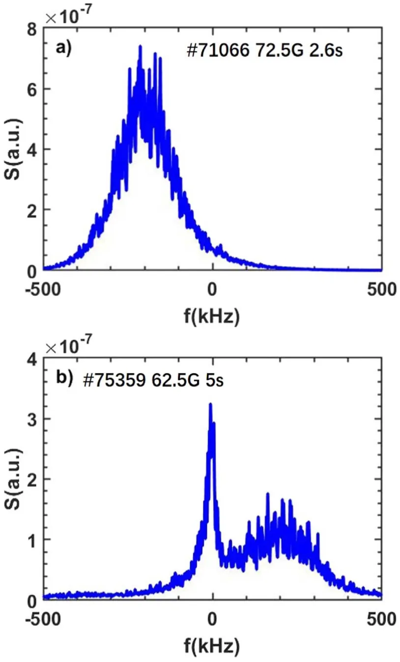
Figure 1.Typical power spectrums of DR.(a) The spectrum with only a Doppler shift peak.(b) The spectrum with a zero-frequency peak and a Doppler shift peak.

Figure 2.SFIT results.(a) The spectrum with only a Doppler shift peak.(b) The DR spectrum with a zero-frequency peak and a Doppler shift peak.

Figure 3.AFIT results.The power spectrum S(f)(black),the mirrored lines S(-f)(red),the asymmetric part S∗(f)(blue),and the fitted lines(purple).(a)The spectrum with only a Doppler shift peak.(b) The spectrum with a zero-frequency peak and a Doppler shift peak.
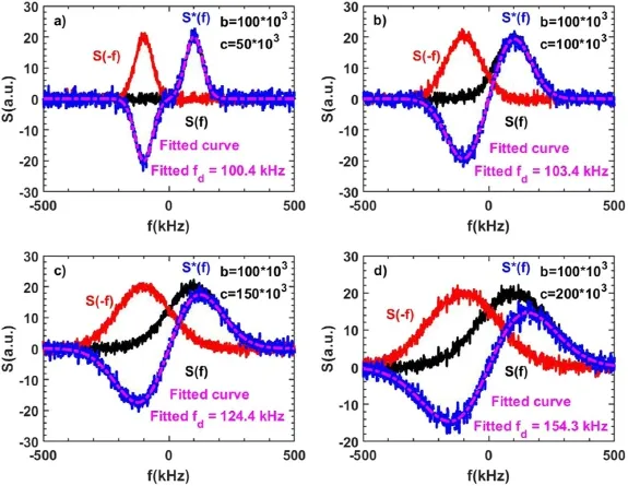
Figure 4.AFIT results for various HWHM.The simulated spectrum S(f)(black),the mirrored lines S(-f)(red),the asymmetric part S∗(f)(blue),and the fitted lines(purple).The Doppler shift is fixed at 100 kHz,and from(a) to(d) the HWHM increase from 50 to 200 kHz.
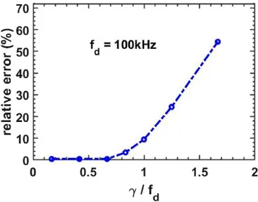
Figure 5.Evolution of the relative error of Doppler shift extracted by AFIT as the HWHM-Doppler shift ratios(γ/fd) increases.The Doppler shift is designed as 100 kHz.
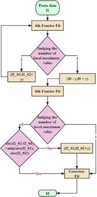
Figure 6.Flowchart of the improved method for extracting Doppler shift.

Figure 7.Process of the improved method for the spectrum with only a Doppler peak.
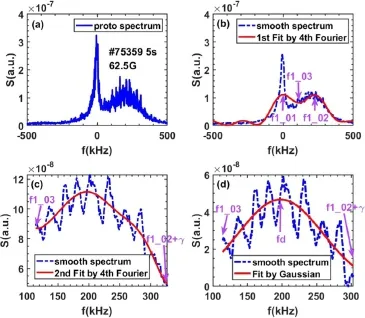
Figure 8.Process of the improved method for the spectrum with a Doppler peak plus a highly visible zero-frequency peak.
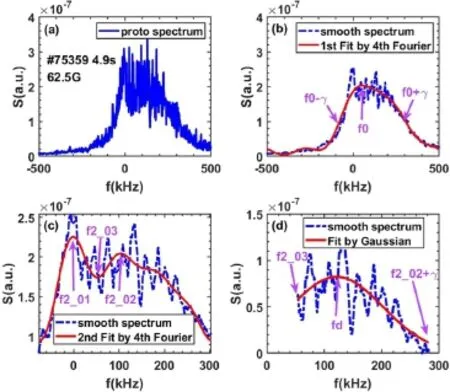
Figure 9.Process of the improved method for the spectrum with a Doppler peak plus an inconspicuous zero-frequency peak.

Figure 10.Process of the improved method for the spectrum with a poor signal-to-noise ratio Doppler peak.
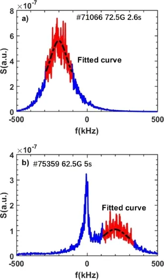
Figure 11.Improved method results.The DR spectrum(blue) and the fitted curves(red).(a) The DR spectrum with only a Doppler shift peak.(b) The DR spectrum with a zero-frequency peak and a Doppler shift peak.
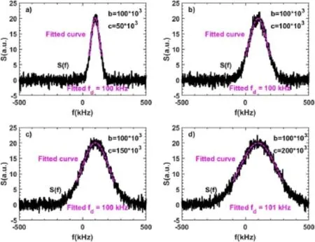
Figure 12.Improved method results for various HWHM.The simulated spectrums S(f) are the same as those in figure 4(black),and the fitted lines are purple.The Doppler shift is fixed at 100 kHz,and from(a) to(d) the HWHM increase from 50 to 200 kHz.
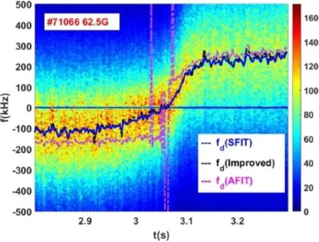
Figure 13.Time-frequency spectrum of a complex signal from the DR.The Doppler shift evolutions were calculated using SFIT(blue)the improved method(black) and AFIT(purple).
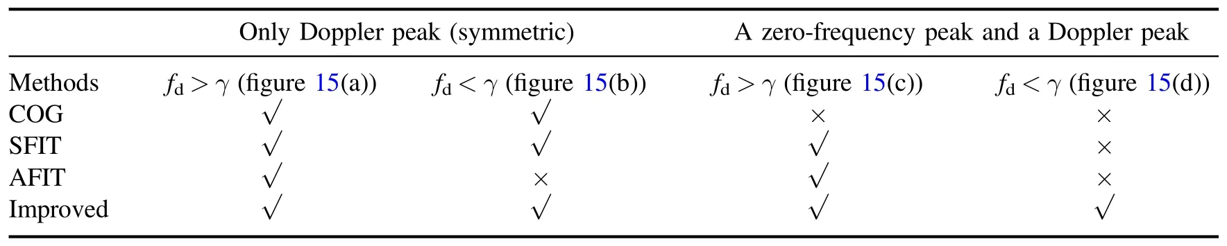
Table 1.The applicability of different methods in various situations.
Figure 14 shows the Doppler shift evolution calculated by various methods for the experimental DR signal.Note that,there is a zero-frequency peak in the DR spectrum,as shown in figures 14(b) and(c).During the time oft=2.95-3.0 s,the Doppler shift calculated by SFIT,AFIT,and the improved method is approximately-220 kHz,while the results of the phase derivative and COG are-120 kHz and-170 kHz,respectively.Beforet=3.12 s,the Doppler shift calculated by the improved method is close to the Doppler shift calculated by AFIT.Aftert=3.14 s,the Doppler shift calculated by the improved method is similar to the Doppler shift calculated by phase derivative,COG,and SFIT.In short,the evolution of the Doppler shift calculated by the improved method has a similar trend with other methods.

Figure 14.(a) Time-frequency spectrum of a complex signal from the DR.The Doppler shift evolutions were calculated using phase derivative(purple),COG(orange),SFIT(red),AFIT(black),and the improved method(blue).(b)Power spectrum in t=3.02 s.(c)Power spectrum in t=3.07 s.
No matter which method is used to calculate the Doppler shift,there will always be errors.In other words,the true Doppler shift(fd)in the experiment cannot be calculated,and all methods are trying hard to get closer to this true Doppler shift.However,in the simulation,we can set the true Doppler shift.Therefore,we can calculate the relative error of the Doppler shift under various methods in the simulation,where the relative error is defined as
Figure 15 illustrates the four DR power spectra in simulation,which can be commonly observed in EAST experimental data,i.e.a Doppler peak withfd>γ(as shown in figure 15(a)),a Doppler peak withfd<γ(as shown in figure 15(b)),a Doppler peak plus a zero-frequency peak withfd>γ(as shown in figure 15(c)),and a Doppler peak plus a zero-frequency peak withfd<γ(as shown in figure 15(d)).In all cases,the HWHM(γ) is set as 100 kHz.For a simulated spectrum with a Doppler peak,the complete spectrum is set aswherebis the true Doppler shift,cis the HWHM(γ).For a simulated spectrum with a Doppler peak plus a zero-frequency peak,the complete spectrum is set aswherebis the true Doppler shift,c1 is the HWHM(γ).Infd>γcases,the true Doppler shift is set as 200 kHz.Infd<γcases,the true Doppler shift is set as 50 kHz.Because the spectrum is not calculated by the proto-time series,the phase derivative method would not be applicable in the simulation.
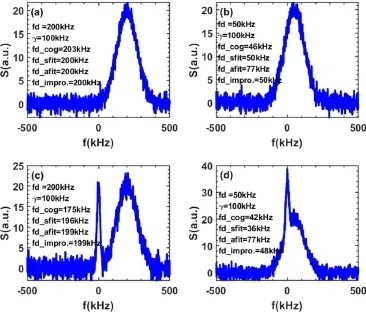
Figure 15.Doppler shift calculated by various methods in different situations.(a) a Doppler peak with fd >γ,(b) a Doppler peak with fd <γ,(c) a Doppler peak plus a zero-frequency peak with fd >γ,(d) a Doppler peak plus a zero-frequency peak with fd <γ.
In figure 15(a),the Doppler shift and the corresponding relative error calculated by COG,SFIT,AFIT,and improved method are 203 kHz(1.5%),200 kHz(0),200 kHz(0),and 200 kHz(0),respectively.In figure 15(b),the Doppler shiftand the corresponding relative error calculated by COG,SFIT,AFIT,and improved method are 46 kHz(8%),50 kHz(0),77 kHz(54%),and 50 kHz(0),respectively.In figure 15(c),the Doppler shift and the corresponding relative error calculated by COG,SFIT,AFIT,and improved method are 175 kHz(12.5%),196 kHz(2%),199 kHz(0.5%),and 199 kHz(0.5%),respectively.In figure 15(d),the Doppler shift and the corresponding relative error calculated by COG,SFIT,AFIT,and improved method are 42 kHz(16%),36 kHz(28%),77 kHz(54%),and 48 kHz(4%),respectively.
In this paper,the relative error of more than 10% is unacceptable.The applicability of different methods in various situations is presented in table 1.It can be found that the AFIT method is not available when the HWHM is larger than the Doppler shift(as shown in figures 15(b)and(d)),and the COG method may have an unacceptable relative error in the spectrum with a zero-frequency peak(as shown in figures 15(c)and(d)).Meanwhile,the SFIT method cannot be employed in the spectrum when the zero-frequency peak exists and the HWHM is larger than the Doppler shift(as shown in figure 15(d)).In short,although all of the commonly used methods for the Doppler shift calculation have their limitations,the improved method can still work reliably even when the zero-frequency peak exists and the HWHM is larger than the Doppler shift.
5.Conclusions
For the Doppler reflectometer,many efforts have been put into the Doppler shift calculation,and different methods are developed in the past years,such as the phase derivative,COG,SFIT,AFIT,and so on.But these methods all have their limitations.The phase derivative,COG,SFIT may give an unaccepted error when the zero-frequency peak exists.Although the AFIT can deal with the zero-frequency peak,it will bring in unacceptable errors when the Doppler shift is relatively small compared to the HWHM.This paper proposes an improved method to extract the Doppler shift.By filtering out the zero-frequency peak and fitting the narrow part around the Doppler shift peak of the spectrum with Gaussian,this improved method can still work reliably even when the zero-frequency peak exists and the HWHM is larger than the Doppler shift.
Acknowledgments
This work was supported in part by the National MCF Energy R&D Program(Nos.2018YFE0311200 and 2017YFE0301204),National Natural Science Foundation of China(Nos.U1967206,11975231 and 11922513).This work was also supported by the Users with Excellence Program of Hefei Science Center CAS(No.2020HSC-UE009).We also acknowledge the EAST team for the aid.
ORCID iDs
 Plasma Science and Technology2023年9期
- Plasma Science and Technology的其它文章
- Plasma-activated hydrogel: fabrication,functionalization,and effective biological model
- Propagation of surface magnetoplasmon polaritons in a symmetric waveguide with two-dimensional electron gas
- Investigation of electron cyclotron wave absorption and current drive in CFETR hybrid scenario plasmas
- Inversion techniques to obtain local rotation velocity and ion temperature profiles for the x-ray crystal spectrometer on EAST
- Impact of resonant magnetic perturbation on blob motion and structure using a gas puff imaging diagnostic on the HL-2A tokamak
- Invariant manifold growth formula in cylindrical coordinates and its application for magnetically confined fusion