A Novel Imaging Method Based on Reweighted Total Variation for an Interferometer Array on Lunar Orbit

Xiaocheng Yang, Mengna Wang, Lin Wu, Jingye Yan, Junbao Zheng, and Li Deng

1 School of Computer Science and Technology, Zhejiang Sci-Tech University, Hangzhou 310018, China 2 Sate Key Laboratory of Space Weather, Chinese Academy of Sciences, Beijing 100190, China; yanjingye@nssc.ac.cn 3 National Space Science Center, Chinese Academy of Sciences, Beijing 100190, China Received 2023 August 2; revised 2023 September 20; accepted 2023 September 22; published 2023 November 15

Abstract Ground-based radio observations below 30 MHz are susceptible to the ionosphere of the Earth and the radio frequency interference.Compared with other space mission concepts,making low frequency observations using an interferometer array on lunar orbit is one of the most feasible ones due to a number of technical and economic advantages.Different from traditional interferometer arrays, the interferometer array on lunar orbit faces some complications such as the three-dimensional distribution of baselines and the changing sky blockage by the Moon.Although the brute-force method based on the linear mapping relationship between the visibilities and the sky temperature can produce satisfactory results in general,there are still large residual errors on account of the loss of the edge information.To obtain the full-sky maps with higher accuracy,in this paper we propose a novel imaging method based on reweighted total variation (RTV) for a lunar orbit interferometer array.Meanwhile, a split Bregman iteration method is introduced to optimize the proposed RTV model so as to decrease the computation time.The simulation results show that, compared with the traditional brute-force method, the RTV regularization method can effectively reduce the reconstruction errors and obtain more accurate sky maps, which proves the effectiveness of the proposed method.

Key words: methods: data analysis – instrumentation: interferometers – techniques: interferometric – space vehicles: instruments – (cosmology:) dark ages – reionization – first stars

1.Introduction

At present, astronomical observations cover the majority of the electromagnetic spectrum from the γ-ray to the radio with only a frequency band basically blank,i.e.,the frequency band below 30 MHz or the wavelengths greater than 10 m.Groundbased radio observations at low frequencies are affected by strong refraction and absorption of the Earth’s ionosphere,and are strongly interfered by artificial radio frequency sources due to internal reflection of the ionosphere.As a result, lowfrequency radio observation below 30 MHz is currently regarded as the last piece of unexplored regime in radio astronomy.

There has been a renewed interest in low-frequency radio astronomy in recent years, particularly motivated by the prospect of observing the redshifted 21 cm line from the cosmic dawn and dark ages (Pritchard & Loeb 2012; Liang et al.2016).For the reasons previously stated, low-frequency radio observations from space are preferable to ground-based observations.From the late 1960s to the 1970s,some satellites,such as the IMP-6 (Brown 1973), and the RAE missions(Alexander & Novaco 1974; Alexander & Kaiser 1975), were launched successively and carried out low-frequency radio observations from space.However, on account of the limitations of the available technology at that time, the resolution of the obtained sky map was so poor that it was difficult to distinguish a single celestial object (Novaco &Brown 1978).On the other hand, the average spectrum of the whole sky measured by different satellites was quite different(Keshet et al.2004).

Note that low frequency radio observations with satellites in Earth orbit are strongly affected by radio frequency interference(RFI)(Zhang et al.2021)from the Earth.In order to overcome the difficulty of the RFI, it is highly desirable to conduct radio observations from the farside lunar surface or on lunar orbit.Although the lunar surface provides a stable platform and can use the Moon to block the interference from the Earth,it brings a series of complex technical problems, such as how to land,how to install and deploy,how to supply the power during the lunar night,and how to transfer data back to the Earth(Cecconi et al.2012; Mimoun et al.2012; Chen et al.2021).

Making low frequency observations by means of the satellites on lunar orbit is one of the most technically and economically feasible solutions at present.On one hand, the Moon effectively blocks the interference from the Earth, and even sometimes the interference from the Sun and planets.On the other hand, the satellite orbits the Moon with a period of about two hours and can use solar cells as the energy.The satellite can transmit the observation data back to the Earth in the arc of the orbit that is not shielded by the Moon,so there is no need for a special relay satellite.Since the 1980s,researchers have proposed a number of space mission concepts of this type,such as the Dark Ages Radio Explorer(Plice et al.2017), the Dark Ages Polarimetry PathfindER (Tauscher et al.2018), Distributed Aperture Array for Radio Astronomy in Space (Boonstra et al.2010) and Discovering the Sky at the Longest wavelength (DSL; (Boonstra et al.2016; Chen et al.2021).

The DSL concept consists of a larger mother satellite and several smaller daughter satellites, forming a linear array orbiting the Moon in nearly the same circular orbit.The purpose of this mission is to perform interferometric imaging to obtain the sky maps below 30 MHz and high-precision global spectral measurements in the frequency range of interest.All daughter satellites are equipped with electrically short antennas for interferometric observations of the sky while they are on the far side of the Moon.The mother satellite will receive the data from the daughter satellites for cross-correlation, store the resulting visibilities and send them back to the Earth when a constellation of satellites are located on the front side of the Moon, i.e., the side facing the Earth.

It is worth noting that the imaging problem of the lunar orbit interferometer array is different from those of the previous ground interferometer arrays and the existing space-ground interferometers such as the HALCA (Frey et al.2000) or RadioAstronA (Kardashev et al.2013).The main complications of the low-frequency interferometer array on lunar orbit are the whole-sky field of view (FOV) for the short dipole antenna array, the three-dimensional (3D) distribution of baselines and the changing part of the sky blocked by the Moon.Considering the actual conditions, the electrically short dipole antennas will be used, which allows the array to have a large FOV, almost covering the whole sky.To ensure that the directional projection aperture and density are basically consistent,the 3D distribution of baselines is generated through the precession of the satellite orbital plane.Moreover, as the satellites orbit the Moon, the part of the sky blocked by the Moon changes over time.

Although the low-frequency interferometer array in lunar orbit has the above-mentioned complications, so long as the visibility data are linearly related to the sky brightness distribution, the interferometric imaging problem in lunar orbit can be regarded as a general linear inversion problem.The brute-force mapmaking method, which has been used in the ground-based MITEoR experiment and obtained satisfactory inverse results (Zheng et al.2017), has been applied to solve the inversion problem (Huang et al.2018; Shi et al.2022).Though the brute-force method produces satisfactory results in general,its disadvantages are no universal method to select the optimal regularization parameter, and the loss of the edge information, which makes residual errors still large.

In recent years, total variation (TV) regularization has been attracting more attention because of its desirable properties such as convexity and the ability to preserve sharp edges(Rudin et al.1992; Vogel & Oman 1998).It has been proved that the TV method is a very effective and efficient algorithm in a wide range of fields, such as image denoising (Yuan et al.2012), image destriping (Chang et al.2013, 2015), computed tomography reconstruction (Tian et al.2011), and reconstruction in synthetic aperture imaging radiometry (Yang et al.2021).Inspired by these, a reweighted total variation (RTV)method based on split Bregman is proposed in this paper to solve the inverse problem for a lunar orbit interferometer array.

This paper is organized as follows.In Section 2, we briefly introduce the general formalism for a lunar orbit interferometer array and the brute-force mapmaking algorithm.In Section 3,we introduce the RTV algorithm based on split Bregman.In Section 4,numerical simulations are performed to illustrate and validate the effectiveness of the proposed method.Finally,some conclusions are drawn in Section 5.

2.Traditional Imaging Algorithm

2.1.Principle of Interferometric Imaging

By measuring the complex correlation between the signals collected by two spatially separated antennas, the interferometers yield the visibility, which could be expressed as

where (u, v, w) are the components of the vector rijin units of wavelength of the radiation, and (l, m, n) are the directional cosine relative to the coordinate axes and l2+m2+n2=1.

For ground-based interferometer arrays with small FOVs,the magnitude of the term w(n-1) is much less than 1, which reduces Equation (2) to an ordinary two-dimensional Fourier transform.As a result,the sky temperature can be reconstructed by a simple inverse Fourier transform.For ground-based interferometer arrays with large FOVs,although the w-term can no longer be ignored,we can still make use of some wide-field imaging algorithms for reconstruction such as the 3D Fourier transform (Perley et al.1989; Cornwell & Perley 1992),faceting (Cornwell & Perley 1992), the W-Projection(Cornwell et al.2008),and W-Stacking(McKinley et al.2015).

However, the above imaging algorithms are not suitable for the low-frequency interferometer array in lunar orbit.The array of short dipole antennas at low frequency produces a large FOV that covers almost the entire sky, rendering the twodimensional Fourier transform method inapplicable.Besides,in order to ensure that the directional projection aperture and density are basically consistent, the 3D distribution of the baseline is produced by the precession of the orbital plane, so an effective 3D algorithm is needed to image the data.Furthermore, the effective blockage fraction of the sky varies when the satellites fly around the Moon, which makes conventional wide-field imaging algorithms inapplicable.In conclusion, we would not be able to solve the interferometric imaging problem in lunar orbit using conventional developed algorithms.

After considering the Moon blockage, Equation (1) is transformed into the following form (Huang et al.2018)

where Sijdenotes the shade function,which describes the timedependent positions in the sky blocked by the Moon.

2.2.Brute-force Mapmaking Algorithm

Despite the complexities described above, the visibility data obtained by the interferometer array on lunar orbit is linearly related to the sky brightness distribution.Furthermore, the brute-force method is used to reconstruct the sky brightness temperature from the measured visibilities.

The integral over sky angles is discretized into a sum over the sky pixels, and Equation (3) can be expressed as

where Npixdenotes the number of pixels, △Ω represents the angular size corresponding to a pixel, and T(n) is the discrete sky map with the aid of the HEALPix scheme (Hansen et al.2006).Moreover,denotes the discrete complex response of the array.

After including the measurement noise, Equation (4) can be rewritten in the matrix form

where V denotes the vector of measured visibilities with the dimension (Nb1·Nt), where Nb1and Ntdenotes the number of baselines and observation time points, respectively.Moreover T is the vector of the sky map with the dimension Npix, B represents the discrete modeling matrix with the dimension(Nb1·Nt)×Npixand the noise vector n has the dimension(Nb1·Nt).

In this paper,the noise is modeled as the Gaussian noise with zero mean and the variance δ2.Assuming that the covariance matrix of the noise is〈nn*〉 =N(∗is the Hermitian conjugate operator), the minimum variance estimator of the sky map is given by

Assuming that the noise is uniform, N is proportional to the identity matrix I.To solve the inverse problem quickly, the singular value decomposition (SVD) of the matrix B is introduced as

where αiand βiare the left and the right singular vectors,respectively, and σiis the singular value of the matrix B in descending order.Due to the fact that very small singular values have a large impact on the error propagation during the reconstruction process, it is preferable to compute the Moore–Penrose pseudoinverse of the matrix B with the aid of the truncated singular value decomposition (Xu 1998)

where m represents the number of singular values retained,namely, the regularization parameter.

2.3.The Regularization Parameter

It should be noted that the selection of the regularization parameter m is of great importance to performance of the bruteforce mapmaking method.The traditional method estimates the regularization parameter according to the threshold ratio(Huang et al.2018).Although it can lead to a stable solution, the value of the threshold ratio is usually set empirically.The disadvantage of the empirical estimation method is that it is easily affected by the personal experience of the estimator and is less precise.

Actually,the choice of the regularization parameter is related to the noise level.However, we usually do not know the information about noise in the real system.In cases where noise cannot be determined, a good way to compute regularization parameters is generalized cross-validation (GCV) criterion(Golub & Matt 1997).The basic idea of the GCV method is that when a component in the original data is removed, that is,an equation is removed from the original linear equation system,the new equation system generated can predict well the removed component.To choose an appropriate regularization parameter, the following functions need to be minimized

where I is the identity matrix,tr(·) denotes the trace of the square matrix,G(λ) =.Consequently, the GCV method is utilized to choose the regularization parameter of the bruteforce approach in this paper.

3.RTV Regularization

The abovementioned brute-force mapmaking method is based on the minimization of the L2norm in the Hilbert space.The TV regularization can better retain the edge information of the image when compared to the L2norm regularization methods.However, owing to the piecewise constant assumption for the image, the traditional TV approach often suffers from over-smoothness on the edges of the image.Consequently,we introduce an RTV regularization method to address the above problem.

According to the regularization theory, the inverse problem(5) can be solved by imposing constraints on the map as follows

where the first term denotes the data fidelity term that provides the similarity between the desired map and reconstructed map,the second term denotes the regularization term, and λ is the regularization parameter aimed at permitting a tradeoff between the data fidelity and regularization terms.For the RTV regularization, the regularization term can be expressed as

where ⊙represents the Hadamard product, ∇represents the gradient operation, and the matrix L denotes the first-order finite-difference operators.Moreover, W denotes a weight vector with the dimension Npixand can be described as follows

where subscript i denotes the pixelʼs index in the map, τ>0 stands for a constant parameter for adjusting the weight and is set to 1 in this paper.Compared with the conventional TV regularization,RTV regularization can effectively reduce oversmoothness and improve the accuracy of the inverse results by assigning different weights to the gradient values at different locations of the map.

The split Bregman iteration algorithm (Cai et al.2010;Goldstein & Osher 2009) is an efficient tool to solve l1-norm regularizations.Compared with conventional optimization methods, the split Bregman method has the advantages ofgood numerical stability and fast convergence speed with less memory usage,which makes it attractive for dealing with largescale problems.As a result, we introduce the split Bregman algorithm to optimize the RTV model.

We introduce an auxiliary variable d=LT and then Equation (10) is equivalent to the constrained problem as

Subsequently, by using the Bregman iteration (Goldstein &Osher 2009),Equation(13)can be converted into the following unconstrained optimization problem

where φ stands for the penalty parameter, b is an auxiliary vector for accelerating the iterations.Obviously,the minimization of(14)with respect to T and d can be decoupled and split,so it can be further transformed into two separate subproblems

The T-related subproblem in Equation(15)is a differentiable optimization problem and can be directly solved by

By using the soft thresholding method proposed in Donoho(1995), Liu et al.(2019), the d-related subproblem in Equation (15) can be solved as

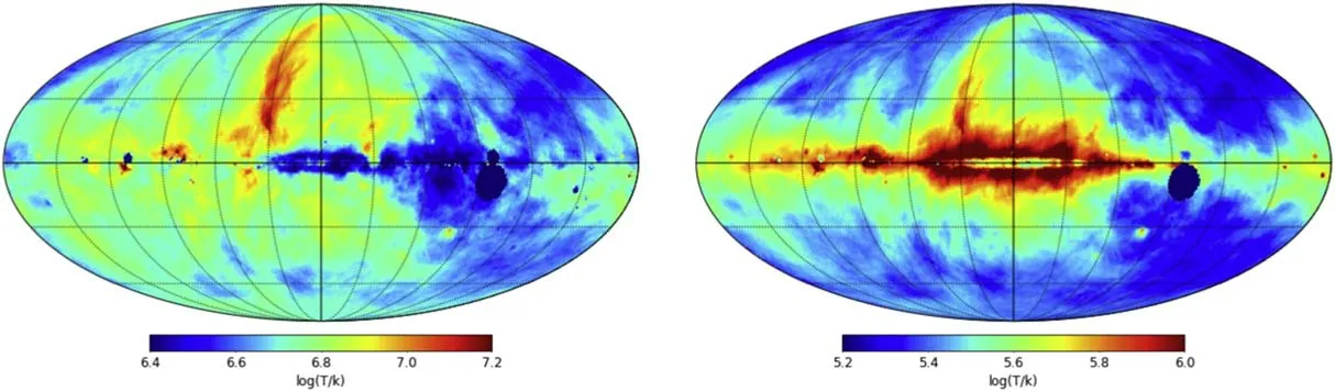
Figure 1.The input full-sky maps at (from left to right) 3 MHz and 10 MHz, respectively.

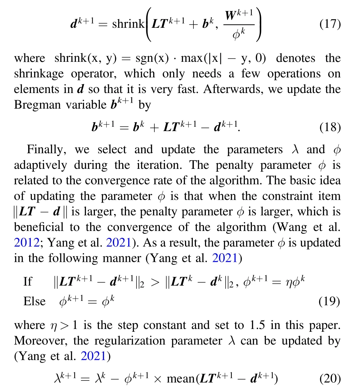
where mean() stands for the mean operator.

In conclusion, the advantage of the split Bregman approach is that the difficult optimization problem is split into two subproblems that are easy to solve.As summarized in Table 1,is the algorithm procedure of the RTV method based on split Bregman.

4.Simulations Results

In this section, numerical simulations have been carried out to discuss and compare the performance of the RTV regularization method with respect to traditional brute-force algorithm developed by Huang et al.(2018).Specifically, we perform full-sky reconstruction, part-sky reconstruction and further analyze the impact of satellite failures.

4.1.Input Sky Map

Currently, the radio sky at the frequency below 30 MHz is barely known.The interpolation/extrapolation of the available data is used in general to generate sky maps at the frequencies without data of surveys.Because sky intensities have an approximate power-law spectrum in most radio bands, the extrapolation is relatively simple and widely used.Researchers have developed a number of extrapolated sky models such as the Global Sky Model(de Oliveira-Costa et al.2008;Rao et al.2017; Zheng et al.2017; Kim et al.2018), and the Selfconsistent Sky Model (Huang et al.2019).However, at the frequency below 10 MHz, due to the lack of observation data and the absorption of the interstellar medium, the extrapolation will become very difficult and complicated.In order to give a reasonable prediction of the sky map below 10 MHz, an Ultralong-wavelength Sky Model with Absorption (ULSA)developed by Cong et al.(2021)takes into account the free–free absorption effect by thermal electrons.Consequently, we generate the input sky map using the ULSA model in this paper.

In the simulations,the sky map is pixelated by the HEALPix(Hansen et al.2006) with Nside=64, which corresponds to 1°pixel size.Figure 1 indicates the input full-sky maps in the logarithmic scale at 3 MHz and 10 MHz, respectively.

4.2.Simulation System

In our simulation, the DSL mission is composed of a larger mother satellite and eight smaller daughter satellites flying around the Moon in the same circular orbit of 300 km height,which is stable enough to avoid the lunar surface due to the irregularity of the Moon’s gravitational field.The daughter satellites equipped with short dipole antennas form a linear interferometer array with a minimum baseline of 1 km and a maximum baseline of 100 km.In addition,the precession of the orbit with an inclination angle of 30° is designed to generate the 3D distribution of the baselines.The orbital plane completes a 360°precession in 1.29 yr.The specific parameters of the DSL system in the simulation are listed in Table 2.

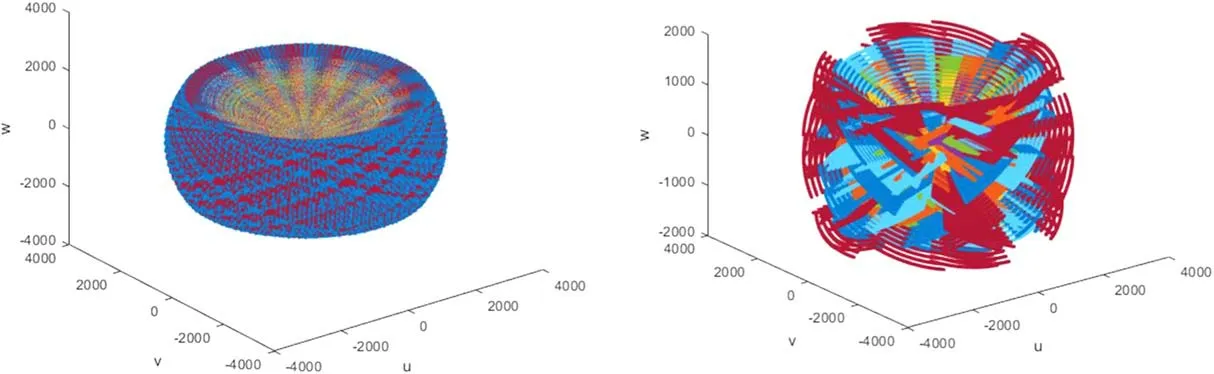
Figure 2.The 3D distributions of cumulative baselines before and after considering the blockage by the Moon (from left to right).

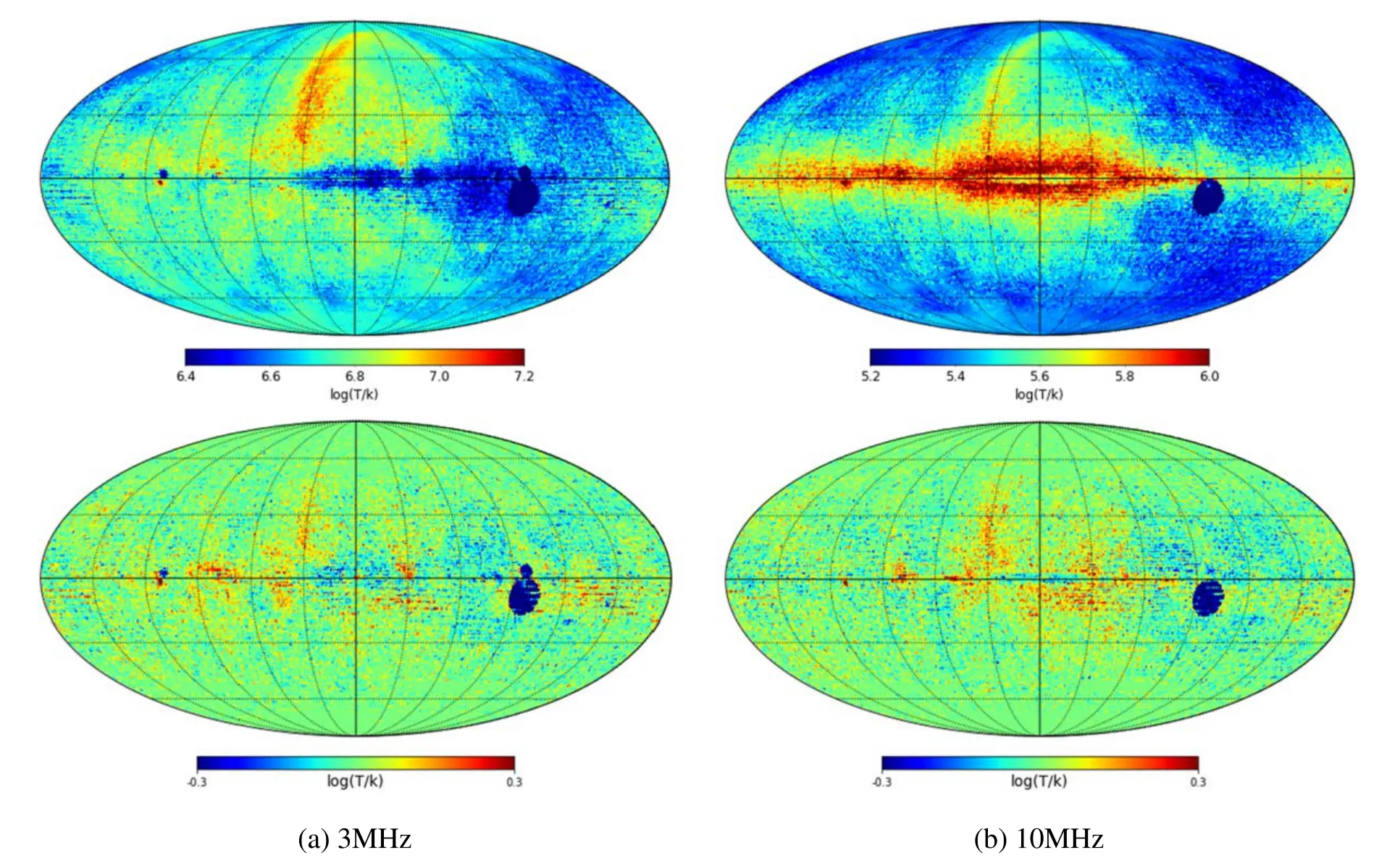
Figure 3.The reconstructed and relative error maps (from top to bottom) for the brute-force method.

Through a precession period, the 3D distribution of cumulative baselines is shown in the left panel of Figure 2.Note that the Moon shields a fraction of the sky when the satellites orbit the Moon.Therefore, in the right panel of Figure 2, we show the 3D distribution of baselines after considering the blockage by the Moon.

Additionally, the Root Mean Squared Error (RMSE) and R-squared (RS) value are calculated to quantitatively analyzethe performance of the imaging methods.The RMSE is defined as

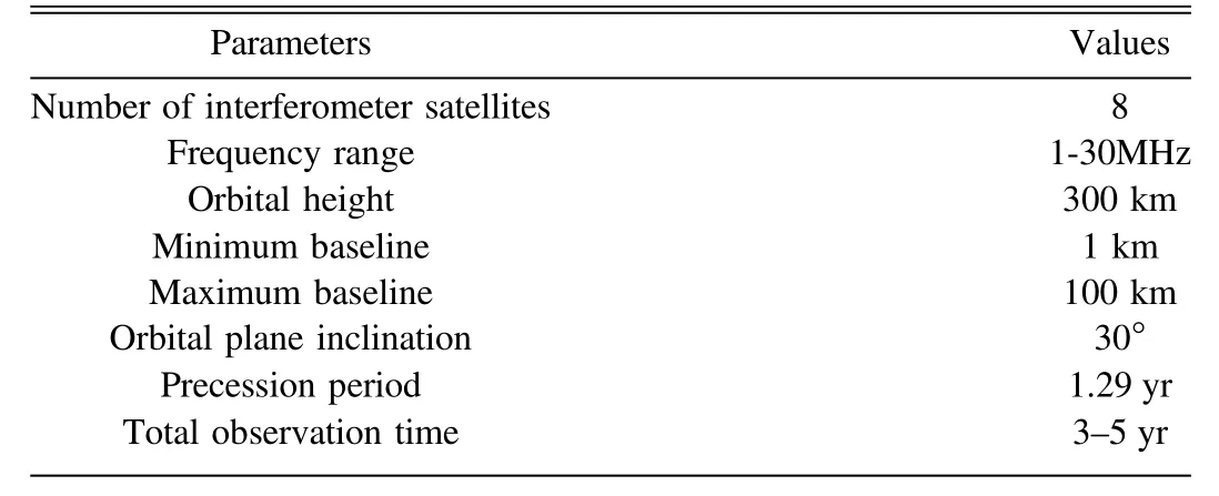
Table 2 Specific Parameters for the DSL System

Figure 4.The reconstructed and relative error maps (from top to bottom) for the RTV method.

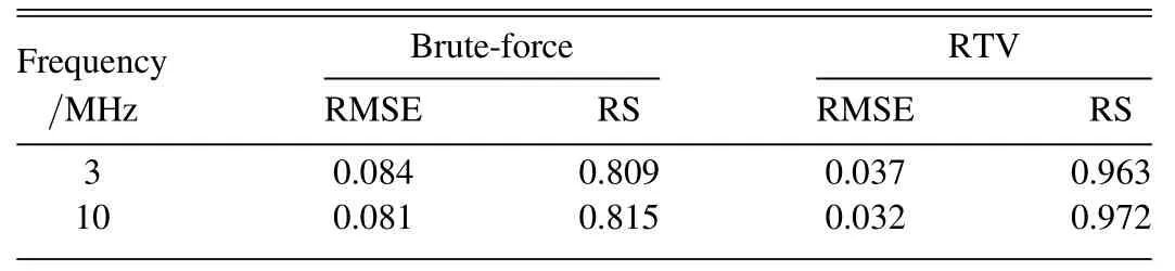
Table 3 Performance Comparison of the Reconstruction Results for Different Approaches

where T(i) anddenote separately the original and reconstructed brightness temperatures.Based on the magnitude of the sky brightness temperatures, the unit of RMSE is set to log10[K ]for the convenience of comparison.The RS is defined aswhererepresents the mean value of the original brightness temperatures.The range of the RS values is (-∞, 1].The closer the RS value is to 1, the closer the reconstructed map is to the actual map.

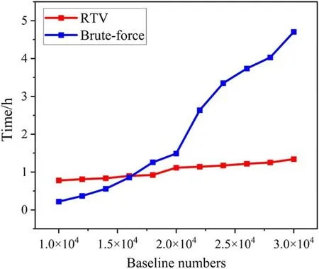
Figure 5.Calculation time of the two methods with different number of baselines.

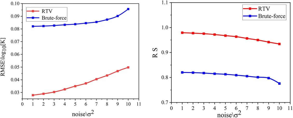
Figure 6.The (from left to right) RMSE and RS values of the two methods under different levels of noise.

4.3.Full-sky Reconstruction

In order to reduce the computation time, in the first experiment we select randomly 3×104points from the total baselines shown in the right panel of Figure 2, which are enough to reconstruct a fairly high-quality sky map at the given angular resolution.According to Equation (5), the measured visibilities are generated by performing forward simulations on the original full-sky maps shown in Figure 1, and the noise is simulated by the Gaussian noise with zero mean and the variance δ2.

In the case of adding the Gaussian noise with the variance δ2=4 (please refer to Equation (35) and Table 4 in Shi et al.2022), the reconstructed full-sky maps and relative error maps at 3 MHz and 10 MHz using the brute-force method are depicted in Figures 3(a)–(b), respectively.The relative error map is defined as the difference between the original map and the reconstructed map.From these results, we can notice that the inversion results for the brute-force method lose a lot of detailed information and exhibit obvious ripples.In addition,Figure 4 shows the full-sky maps at 3 and 10 MHz reconstructed using the RTV method.It can be observed that the RTV method produces satisfactory reconstruction results,which can match the actual maps well.Compared to the bruteforce method, the inversion results for the RTV method are visually better and smoother with clearer edges and details.

For the purpose of quantitatively evaluating the performance of the reconstruction results for the aforementioned two approaches, we calculate the RMSE and RS values, which are listed in Table 3.The results witness that the performance of the RTV approach is markedly better than that of the bruteforce approach, since the RTV approach has obviously lower RMSE and higher RS values.As a result, the RTV approach can more effectively reduce the reconstruction errors than the brute-force approach.

Moreover, we compare the computation speed of the bruteforce and RTV algorithms.As an iterative method, the computation time of the RTV algorithm is mainly related to the size of the modeling matrix B and the iteration steps.For the reconstructed maps shown earlier, the MATLAB runtime(MATLAB R2020b on a PC with Intel Core i9-9900k processor and 64 GB RAM) of the brute-force algorithm is 4.703h, whereas the MATLAB runtime of the RTV algorithm is 1.307h when the size of B is 30,000×49,152 and the number of iterations is 10.The results reveal that the computation time of the RTV algorithm is distinctly lower than that of the brute-force algorithm.To further improve the calculation speed,the RTV algorithm could run on the graphics processing unit platform in the future.

Figure 5 shows the calculation time of the brute-force and RTV methods with different numbers of baselines.It can be noticed that as the number of the baselines increases, the calculation time of the brute-force method goes up rapidly,while that of the RTV method augments slowly.This is because the computation time of the brute-force method is mainly derived from the SVD of the modeling matrix B, the time of which will augment significantly with the increase of the matrix size.In contrast, the calculation time of the RTV method mainly derives from the iterative solution process,which has been accelerated by means of the split Bregman algorithm.As a consequence, from the perspective of the computation speed, the RTV method performs better than the brute-force method when the number of baselines is large.

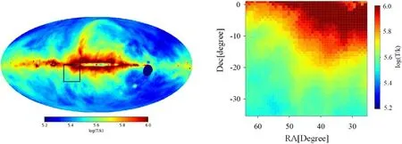
Figure 7.The original part-sky map and the position in the full-sky map (from left to right).

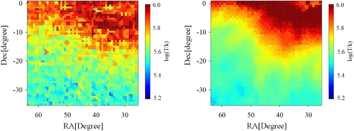
Figure 8.The retrieved part-sky maps for (from left to right) the brute-force and RTV approaches.

Furthermore, we analyze the impact of noise on the performance of the reconstruction methods.The full-sky map at 10 MHz generated by the ULSA model(Cong et al.2021)is selected as the input sky map, as shown in the right panel of Figure 1.The measured visibilities blurred by the zero mean Gaussian noise with different variance are used to retrieve the sky maps.In Figure 6, we show the RMSE and RS values of the two methods under different levels of noise,respectively.It can be noted from Figure 6 that the RTV approach has an evident RMSE reduction and an apparent RS improvement over the brute-force approach, although the noise level varies.To be more specific, the reduction of the RMSE value is more than 60%and the increase of the RS value is more than 16%for the RTV approach with respect to the nominal brute-force approach.This indicates that compared with the brute-force approach, the RTV approach is more robust to the noise interference.

4.4.Part-sky Reconstruction

In order to illustrate even more the comparison between the two approaches, we implement the second experiment, where the simulation is limited to a small part of the full-sky map.Because there are huge amounts of pixels in the full-sky map,the calculated amount required to retrieving the full-sky map is quite huge and unaffordable.In consequence, to immensely reduce the computational load, the part-sky reconstruction has been introduced and proved to be feasible in Shi et al.(2022).Here,we apply the part-sky reconstruction to test and ascertain the effectiveness of the RTV approach.

Figure 9.Cumulative baseline distribution over two months.

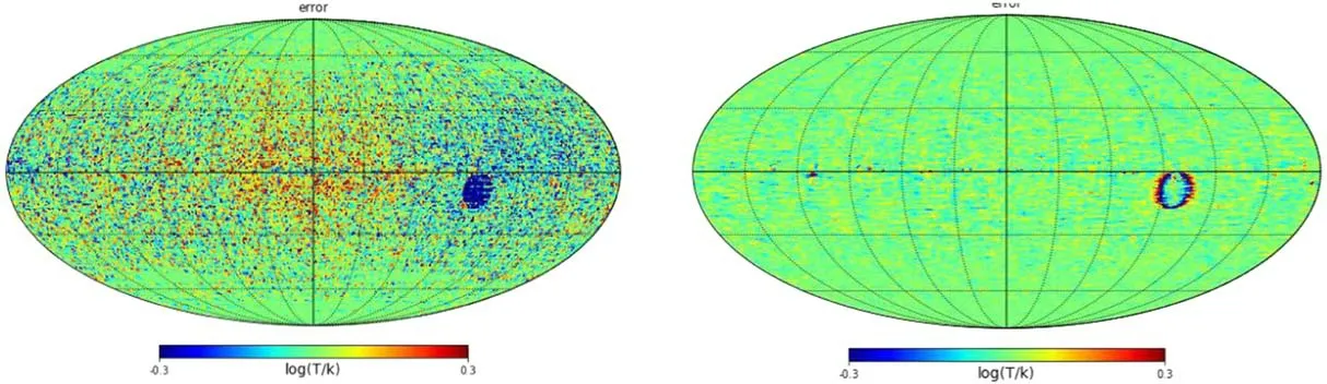
Figure 10.The relative error maps for the brute-force and RTV methods (from left to right).

From the full-sky map with 1° resolution at 10 MHz, we choose a black rectangular area (R.A.(R.A.): [65°, 25°], decl.(decl.): [-35°, 0°]) as the original part-sky map, as shown in Figure 7.Under the same observation conditions as the full-sky reconstruction in Section 4.2, the retrieved part-sky maps via the brute-force and RTV approaches are shown in Figure 8.One can notice that the brute-force algorithm gives rise to the reconstruction results that have obvious oscillation ripples.Besides, compared with the brute-force algorithm, the RTV algorithm results in an excellent inversion result with weaker oscillation ripples,which is in better agreement to the reference part-sky map.

The RMSE and RS values related to the retrieved part-sky maps are calculated to analyze the reconstruction errors quantitatively.The RMSE values for the brute-force and RTV approaches are separately 0.156 and 0.053 log10[K ], and the RS values for the brute-force and RTV approaches are 0.808 and 0.978, respectively.The results reveal that the RTV approach has better performance, compared to the brute-force approach.Therefore,the RTV approach can better improve the accuracy of the reconstruction results when compared to the brute-force approach.

4.5.The Impact of Satellite Failures

In this subsection, we consider the reconstruction accuracy of the sky map under situation in the absence of visibility data due to satellite failures.In practice, such hardware failures are often unpredictable and probably occur (Yan et al.2023).The parameters of the simulation system have been shown in Section 4.2, but we consider that the satellite failures occur after the system only operates healthily for two months.The cumulative baseline distribution over two months is shown in Figure 9, where there are 47,100 points.

The input map has been shown in the right panel of Figure 1.When the variance of the additive Gaussian noise is equal to δ2=4, the relative error maps are presented in Figure 10 via the brute-force and RTV methods.The results reveal that there are still large reconstruction errors for the maps reconstructed by the brute-force method.In contrast,the reconstruction errors for the RTV method are considerably diminished.

Moreover, we calculate the RMSE and RS values to quantitatively appraise the performance of the reconstructed results.The RMSE and RS values for the brute-force method are 0.124 log10[K ] and 0.592, respectively.In contrast, the RMSE and RS values for the RTV method are 0.044 log10[K ]and 0.949,respectively.The results witness that compared with the brute-force method, the RTV method can effectively diminish the reconstruction errors even in the case of satellite failures.

5.Conclusions

At present,low-frequency radio observations below 30 MHz are considered as the final unexplored window in radio astronomy.Ground-based radio observations below 30 MHz are hindered by the refraction and absorption of the Earthʼs ionosphere, and the RFI.In consequence, making low frequency observations from space as a better choice has become a research hotspot.Compared with other space mission concepts, an interferometer array on lunar orbit is one of the most technically and economically feasible ones.

Different from traditional interferometer arrays, the interferometer array in lunar orbit faces some complications such as the whole-sky FOV for the short dipole antenna array, the 3D distribution of baselines,and the changing sky blockage by the Moon.Despite these complexities,the relationship between the visibilities and the sky brightness temperature can be expressed as the linear mapping equations.Furthermore, the brute-force method is introduced to solve the linear inversion problem and obtain the sky map.However,the brute-force method could not preserve well the edge information of the sky map,resulting in large residual errors.

In order to obtain the full-sky maps with higher accuracy,we propose a novel RTV approach to solve the inverse problem for a lunar orbit interferometer array.Meanwhile,we introduce the split Bregman iteration method to optimize the RTV regularization model so as to increase the computation speed of the reconstruction process.The simulation results show that,compared with the traditional brute-force method, the RTV regularization method can more effectively reduce reconstruction errors and obtain more accurate full-sky maps, which proves the effectiveness of the proposed method.

In the presented simulations,we neglect some practical issues,such as calibration errors and measurement errors at the baselines.In future works,we shall conduct an end-to-end simulation using all the baselines and the input full-sky maps with the nominal resolution while considering these practical issues.

Acknowledgments

This work is supported by the Specialized Research Fund for State Key Laboratories under Grant 202217 and the Key Laboratory of Solar Activity and Space Weather(NSSC)under Grant E26600021S.

ORCID iDs