A Revised Graduated Cylindrical Shell Model and its Application to a Prominence Eruption

Qing-Min Zhang, Zhen-Yong Hou, and Xian-Yong Bai

1 Key Laboratory of Dark Matter and Space Astronomy, Purple Mountain Observatory, Nanjing 210023, China; zhangqm@pmo.ac.cn 2 Yunnan Key Laboratory of the Solar Physics and Space Science, Kunming 650216, China 3 School of Earth and Space Sciences, Peking University, Beijing 100871, China 4 National Astronomical Observatories, Chinese Academy of Sciences, Beijing 100101, China 5 University of Chinese Academy of Sciences, Beijing 100049, China 6 Key Laboratory of Solar Activity and Space Weather, National Space Science Center, Chinese Academy of Sciences, Beijing 100190, China Received 2023 May 21; accepted 2023 July 3; published 2023 October 25

Abstract In this paper,the well-known graduated cylindrical shell(GCS)model is slightly revised by introducing longitudinal and latitudinal deflections of prominences originating from active regions (ARs).Subsequently, it is applied to the three-dimensional(3D)reconstruction of an eruptive prominence in AR 13110,which produced an M1.7 class flare and a fast coronal mass ejection (CME) on 2022 September 23.It is revealed that the prominence undergoes acceleration from ∼246 to ∼708 km s−1.Meanwhile,the prominence experiences southward deflection by 15°±1°without longitudinal deflection, suggesting that the prominence erupts non-radially.Southward deflections of the prominence and associated CME are consistent, validating the results of fitting using the revised GCS model.Besides, the true speed of the CME is calculated to be 1637±15 km s−1, which is ∼2.3 times higher than that of prominence.This is indicative of continuing acceleration of the prominence during which flare magnetic reconnection reaches maximum beneath the erupting prominence.Hence, the reconstruction using the revised GCS model could successfully track a prominence in its early phase of evolution, including acceleration and deflection.

Key words: Sun: flares – Sun: filaments – prominences – Sun: coronal mass ejections (CMEs)Supporting material: animation

1.Introduction

Solar flares and coronal mass ejections (CMEs) are the most powerful activities in the solar atmosphere, which have drastic and profound influences on the heliosphere(Chen 2011;Shibata& Magara 2011; Reames 2013).The primary origins of flares and CMEs are believed to be impulsive eruptions of solar prominences or filaments (Janvier et al.2015).Prominences observed in Hα or extreme-ultraviolet (EUV) wavelengths usually show helical structures (Kumar et al.2012), and fast rotations or untwisting motions are frequently detected during eruptions (Green et al.2007; Yan et al.2014; Shen et al.2019;Zhou et al.2023).Before loss of equilibrium, the gravity of a prominence is balanced by the upward tension force of magnetic dips within a sheared arcade or a flux rope(Liu et al.2012;Chen et al.2018; Zhou et al.2018; Luna & Moreno-Insertis 2021;Guo et al.2022).A magnetic flux rope comprises a bundle of twisted field lines, which are wrapping around a common axis(Titov & Démoulin 1999; Qiu et al.2004; Wang et al.2015;Gou et al.2023).Flux ropes play a central role in driving flares and CMEs (Amari et al.2003; Roussev et al.2003; Aulanier et al.2010;Cheng et al.2013;Inoue et al.2018;Mei et al.2020;Jiang et al.2021).Sometimes, they could be heated up to∼10 MK before or during eruptions and are termed as hot channels (Zhang et al.2012; Cheng et al.2013; Zhang et al.2022b; Liu et al.2022), which are merely observed in 94 and 131 Å of the Atmospheric Imaging Assembly (AIA; Lemen et al.2012) on board the Solar Dynamics Observatory (SDO)spacecraft.Flux ropes propagate radially in most cases.However, a fraction of them undergo deflections and propagate non-radially (Guo et al.2019; Mitra & Joshi 2019; Hess et al.2020;Zhang et al.2022a).The inclination angle with the normal direction lies in the range of 15°–70°.In the typical three-part structure of CMEs, the dark cavity and bright core are considered to be a flux rope and the embedded prominence(Illing & Hundhausen 1985; Song et al.2023).

The three-dimensional (3D) shape and direction of a CME are essential in estimating the arrival time and geo-effectiveness of a CME.The well-known cone model,resembling an ice cream, was proposed and applied to investigate the evolutions of morphology and kinematics of halo CMEs (Michałek et al.2003; Xie et al.2004).This model assumes a constant angular width and a constant linear speed during propagation in the radial direction (Zhang et al.2010).Considering that a part of prominences and the driven CMEs propagate non-radially,Zhang (2021) put forward a revised cone model and applied it to two prominence eruptions.The tip of the cone is located at the source region of CME.The model is characterized by four parameters: the length (r) and angular width (ω) of the cone,and two angles (φ1and θ1) denoting the deflections in the longitudinal and latitudinal directions.Using this model,Zhang(2022)satisfactorily tracked the 3D evolution of a halo CME as far as ∼12 R⊙on 2011 June 21.

Figure 1.(a) Positions of Earth(green circle) and two artificial satellites.SAT-1(maroon circle) and SAT-2(purple circle) have separation angles of −15° and 90°with the Sun-Earth connection,respectively.(b)Positions of Earth(green circle),ahead STEREO(STA,maroon circle),and behind STEREO(STB,purple circle)on 2022 September 23.

Thernisien et al.(2006) proposed the graduated cylindrical shell(GCS)model to perform 3D reconstructions of flux ropelike CMEs(Vourlidas et al.2013).The flux rope in their model looks like a croissant, which has two identical legs with a length of h and angular separation of 2α (Thernisien et al.2009; Thernisien 2011).The legs are connected by a circulus with varying cross sections so that the aspect ratio κ keeps constant.Another angle γ represents the tilt angle of the polarity inversion line (PIL) of the source region with a longitude φ and a latitude θ, respectively.Besides, electron number density (Ne) is considered to synthesize white-light(WL) images observed by coronagraphs.Thanks to multiperspective observations from the Large Angle and Spectrometric Coronagraph(LASCO;Brueckner et al.1995)on board the SOHO spacecraft and WL coronagraphs(COR1,COR2)on board the twin Solar TErrestrial RElations Observatory(STEREO; Kaiser et al.2008) spacecraft, the GCS model has been widely used to perform 3D reconstructions of CMEs(Mierla et al.2009; Cheng et al.2014; Möstl et al.2014;Liewer et al.2015; Lu et al.2017; Sahade et al.2023; Zhou et al.2023).Isavnin(2016)developed an analytic 3D model for flux rope-like CMEs that incorporate all major deformations during their propagations, such as deflection, rotation,“pancaking,” front flattening, and skewing.

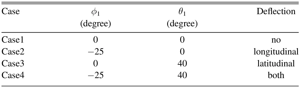
Table 1Parameters of φ1 and θ1 in Four Cases

The 3D morphologies of eruptive prominences could be obtained using the triangulation technique when simultaneous observations from two or three perspectives are available(Thompson 2009; Li et al.2011; Bi et al.2013; Guo et al.2019).Deflection,kinking,and rotation of the prominences are found based on the 3D reconstruction.Until now, the GCS model has rarely been applied to the reconstruction of eruptive prominences,especially those propagating non-radially.In this paper, the GCS model is slightly modified and applied to reconstruct the shapes of an eruptive prominence in NOAA active region (AR) 13110(N16E84), which produced a GOES M1.7 class flare and a fast CME on 2022 September 23.The model is described in Section 2.The results of 3D reconstruction are presented in Section 3.A brief summary and discussions are given in Section 4.

2.Revised GCS Model

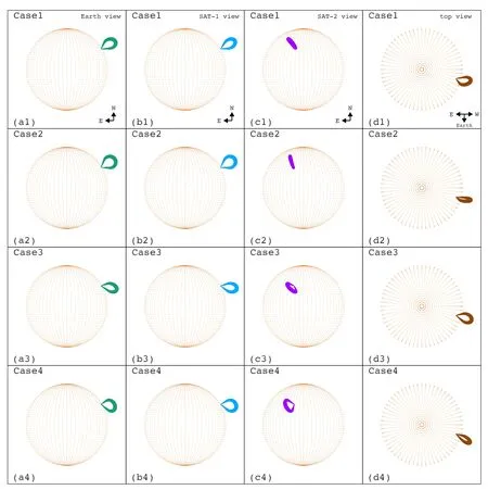
Figure 2.Different views of four artificial flux ropes (Case1−Case4) in the revised GCS model, see text for details.

Similar to the revised cone model, the GCS model is also modified in two aspects:First,the tip of the two legs is located at the source region of the eruptive prominence rather than the solar center.This applies to flux ropes originating from active regions, instead of quiescent prominences with much longer extensions(Li et al.2011;Dai et al.2021;Zhou et al.2023).It should be emphasized that the footpoints of a flux rope have separation and are not strictly close to each other (Wang et al.2015).Moreover, the footpoints may experience long-distance migration during eruption(Gou et al.2023).In this respect,the assumption that the footpoints of a flux rope are cospatial is relatively strong.Second, the GCS symmetry axis passing through the circulus has inclination angles of φ1and θ1with respect to the local longitude and latitude, respectively.The parameters h, α, κ, γ, φ, and θ have the same meanings(Thernisien et al.2006).γ=0° and γ=90° indicate that the PIL is parallel and perpendicular to the longitude,respectively.Since the traditional GCS model reduces to the ice cream cone model when α=0 (Thernisien et al.2009), the revised GCS model also reduces to the revised cone model when α=0(Zhang 2021).

The transform between the heliocentric coordinate system(HCS;Xh,Yh,Zh)and local coordinate system(LCS;Xl,Yl,Zl)is (Zhang 2022):

where

Figure 3.(a)GOES SXR light curves of the M1.7 flare in 1−8 Å(red line)and 0.5−4 Å(purple line).The dashed–dotted line marks the peak time(18:10:00 UT).(b)Height-time plots of the leading edges of the reconstructed flux rope(blue circles)and CME observed by STA/COR2(green diamonds).(c)Height-time plots of 3h(brown squares)and hLE(dark cyan squares).Linear fittings of hLE are performed before and after 17:53:00 UT,with the speeds being labeled.(d)Time variations of the fitted parameters, including 90 −γ (green rhombuses), ωFO/2 (purple triangles), α (orange squares), θ1 (yellow circles), ωEO (yellow triangles), and φ1 (gray hexagons), respectively.

The transform between LCS and GCS flux-rope coordinate system (FCS; Xf, Yf, Zf) is:

where

To reconstruct the shape of a flux rope in the revised model,observations from multiple viewpoints are needed as far as possible.In Figure 1(a),the relative positions of Earth and two artificial satellites (SAT-1 and SAT-2) are denoted with green,maroon,and purple circles,respectively.The separation angles between the artificial satellites with the Sun-Earth connection are denoted by ξ1and ξ2, respectively.Note that SAT-1 and SAT-2 could be the ahead STEREO (hereafter STA) and behind STEREO (hereafter STB), or Extreme-Ultraviolet Imager (EUVI; Rochus et al.2020) on board Solar Orbiter(SolO; Müller et al.2020), or Wide-Field Imager for Solar Probe Plus (WISPR; Vourlidas et al.2016) on board Parker Solar Probe (PSP; Fox et al.2016).Note that both SolO and PSP are much closer to the Sun than STEREO.Consequently,the transform between the SAT-1 coordinate system (Xs1, Ys1,

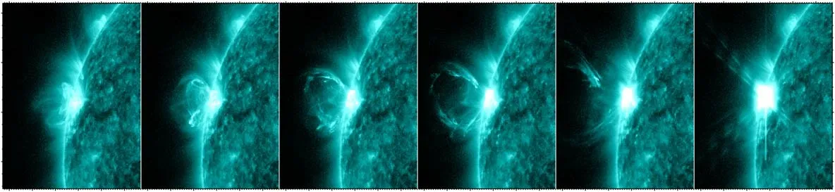
Figure 4.AIA 131 Å images to illustrate the evolutions of the prominence and flare.The white arrows point to AR 13110,eruptive prominence,and hot flare loops.An animation showing the flare and prominence eruption in AIA 131 Å is available.It covers a duration of 50 minutes from 17:30 UT to 18:20 UT on 2022 September 23.The entire movie runs for 6 s.

Zs1) and HCS is:

where

Similarly, the transform between the SAT-2 coordinate system (Xs2, Ys2, Zs2) and HCS is:

where

3.Application to a Prominence Eruption

3.1.Flare and CME

The event occurred in AR 13110, accompanied by an M1.7 flare and a fast CME.Figure 3(a) shows SXR light curves of the flare in 1–8 Å(red line)and 0.5–4 Å(purple line).The SXR emissions increase from 17:48:00 UT, peak at 18:10:00 UT,and decrease slowly until ∼18:50:00 UT.Time evolutions of the prominence eruption and flare are illustrated by six 131 Å images observed by SDO/AIA in Figure 4 and the associated online movie (anim131.mp4).Panel (a) shows AR 13110 with weak brightening before eruption.The prominence shows up and stands out after ∼17:46:00 UT (panel (b)).It continues to rise and expands in height, during which the flare loops brighten significantly (panels (c)–(d)).The prominence accelerates and the apex escapes the field of view (FOV) of AIA,leaving behind the hot post-flare loops that cool down gradually (panels (e)–(f)).It is noticed that the footpoints of the prominence remain in the AR without considerable separation.The morphological evolution of the prominence is similar in other EUV and 1600 Å wavelengths of AIA,indicating its multithermal nature (Zhang et al.2022a; Li et al.2022b).

Figure 5.(a)–(c) Running-difference images of the related CME observed by LASCO/C2 during 18:12−18:36 UT.(d)–(i) Running-difference images of the CME observed by STA/COR2.The arrows point to the CME that first appears in the coronagraphs.

In Figure 5, the top panels show running-difference WL images of the related CME observed by LASCO/C2.The CME7www.sidc.be/cactus/first appears at 18:12:00 UT and propagates eastward with an angular width of ∼50°and at a speed of ∼1644 km s−1(see Table 2).It is worth mentioning that the angular width is measured for the CME itself.Since an interplanetary shock wave was driven by the CME (Figures 5(b)–(c)), the recorded angular width of the CME reaches 189°, which is much wider than the CME itself.8cdaw.gsfc.nasa.gov/CME_list/UNIVERSAL_ver1/2022_09/univ2022_09.htmlIn Figure 1(b), the green, maroon, and purple circles represent the positions of Earth, STA, and STB on 2022 September 23.The twin satellites had separation angles of −17.9° and 12.9° with the Sun-Earth connection,although STB stopped working after 2016.The middle and bottom panels of Figure 5 show running-difference images of STA/COR2 during 18:23−19:38 UT.The CME enters the FOV of COR2 at 18:23:30 UT and propagates eastward with an angular width of ∼64° (see Table 2).The height evolution of the CME leading edge in the FOV of COR2 is plotted with green diamonds in Figure 3(b).A linear fitting results in an apparent speed of ∼1482 km s−1.

3.2.3D Shapes of the Prominence

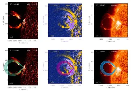
Figure 6.Top panels: the prominence observed by AIA 304 Å (a1), SWAP 174 Å (b1), and EUVI 304 Å (c1) passbands around 17:55:40 UT.Bottom panels: the same images superposed with projections of the reconstructed flux rope (atrovirens, magenta, and blue dots).

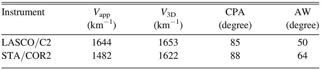
Table2 Parameters of the CME Produced by the Prominence Eruption, Including the Apparent Speed (Vapp), True Speed (V3D), Central Position Angle (CPA), and Angular Width (AW)

In Figure 6, the top panels show the prominence simultaneously observed by AIA 304(base-difference image),SWAP 174(base-difference image), and EUVI 304(original image) passbands around 17:55:40 UT.Due to the low cadence(10 minutes)of EUVI 304passband,this is the only time when the prominence is entirely visible in all instruments.Owing to the smaller FOV of AIA than SWAP and EUVI, the whole prominence was captured by SWAP and EUVI, while the outermost part (i.e., apex) of the prominence was missed by AIA.It is obvious that the two legs are much brighter than the top of the prominence.In panel (c1), the prominence presents clear helical structure, implying that the magnetic fields supporting the prominence are most probably a flux rope.The bottom panels of Figure 6 show the same images, which are superposed with projections of the reconstructed flux rope (atrovirens, magenta, and blue dots)using the revised GCS model.The 3D reconstruction is performed by repeatedly adjusting the free parameters described in Section 2, while the source region location(φ=−84°,θ=15°)is fixed.The best-fit model is subjectively judged when projections of the flux rope nicely match the prominence in EUV images.From Figures 6(a2)–(c2), it is revealed that the fitting of the prominence using the revised GCS model is satisfactory.The derived parameters are:h=150″, α=45°, κ=0.087 (δ=5°), φ1=0°, θ1=16°, andedge-on width of the flux rope is ωEO=2δ=10°,and the faceon angular width is ωFO=2(α+δ)=100°.The flux rope axis deviates from the local vertical direction by 16° and the heliocentric distance (hHC) of the leading edge reaches∼1.4 R⊙.

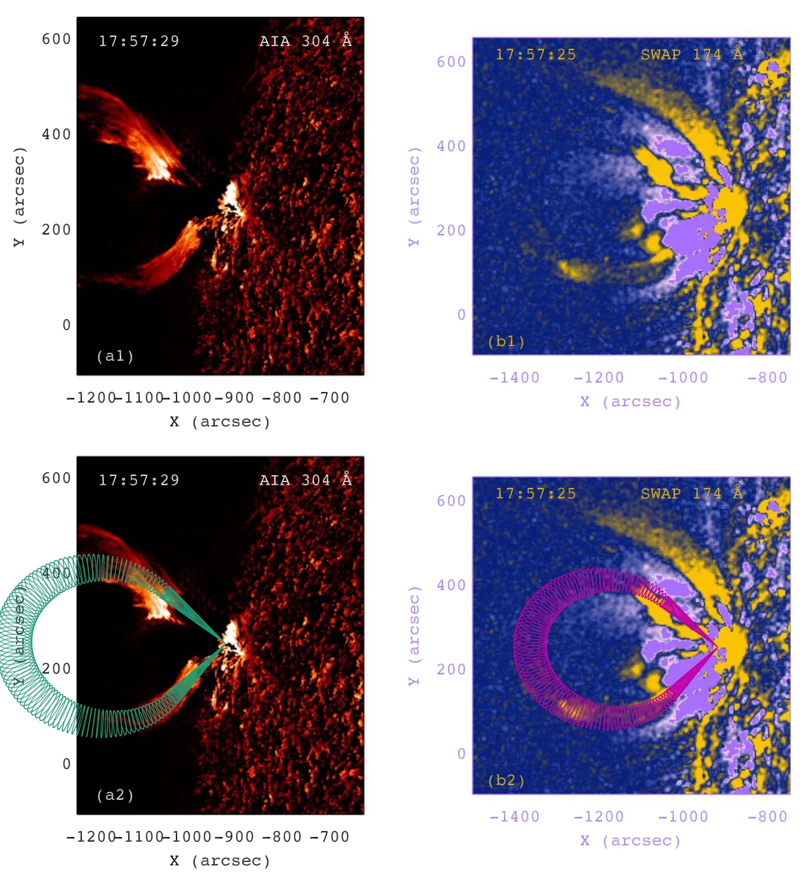
Figure 7.Top panels:the prominence observed by AIA 304 Å and SWAP 174 Å around 17:57:27 UT.Bottom panels:the same images overlaid with projections of reconstructed flux rope (atrovirens and magenta dots).

Although there is only one time of simultaneous observations of the prominence from multiple perspectives, 3D reconstruction could still be conducted using observations of telescopes along the Sun-Earth connection (Thernisien et al.2006).In Figure 7, the top panels show the prominence observed by AIA 304 Å and SWAP 174 Å around 17:57:27 UT.The prominence was fully visible in SWAP 174 Å image at 17:57:25 UT, but was partly visible in AIA 304 Å image at 17:57:29 UT.The bottom panels show the same images overlaid with projections of reconstructed flux ropes(atrovirens and magenta dots).Consistency between the shapes of prominence and flux ropes indicates that the fittings are still gratifying.The derived parameters are drawn in Figures 3(c)–(d).

Before 17:54:00 UT, the prominence rose gradually and was entirely recorded in AIA 304 Å and SUTRI 465 Å passbands.Figure 8 shows 304 Å images(a1–a5)and 465 Å images(b1–b5)overlaid with projections of the reconstructed flux ropes(atrovirens and blue dots) during 17:49–17:53 UT.The prominence looks like an ear and the two legs are much clearer than the top.The reconstructed flux ropes coincide with the prominence much better at the legs than the top due to its irregular and asymmetric shape.The derived parameters are drawn in Figures 3(c)–(d).Linear fittings of hLEare separately performed during 17:49:17–17:52:17 UT and 17:53:30–17:57:30 UT,giving rise to true speeds of ∼246 and ∼708 km s−1of the erupting prominence.Accordingly, the prominence was undergoing acceleration during its early phase of eruption(17:49–17:57 UT).In Figure 3(b), time variation of hHCis plotted with blue circles, which has the same trend as hLE.

Figure 8.AIA 304 Å images(a1–a5)and SUTRI 465 Å images(b1–b5)superposed with projections of the reconstructed flux ropes(atrovirens and blue dots)during 17:49−17:53 UT.

The value of γ increases from 0° to 30°, which is probably indicative of counterclockwise rotation of the prominence axis during eruption (Fan & Gibson 2003; Zhou et al.2020).The edge-on width ωEOkeeps a constant of ∼10°.The face-on width ωFOdecreases from ∼162° to a minimum of ∼100°around 17:53:45 UT and increases to ∼104° around 17:57:25 UT.The inclination angle θ1increases slightly from 14°to 16°,suggesting a southward deflection of the prominence.The values of φ1remain 0°, meaning that there is no longitudinal deflection.In Table 2,the CPA of CME is 85°–88°,indicating a southward deflection of CME by 11°–14°.In this regard,deflections of the prominence and related CME are accordant,which justifies the results of fitting using the revised GCS model.Furthermore, the true speeds (V3D) of CME are estimated to be 1653 and 1622 km s−1using the apparent speeds in the FOVs of LASCO/C2 and STA/COR2,which are very close to each other.It is noted that the speed of CME(1637±15 km s−1) is ∼2.3 times higher than that of prominence, implying continuing acceleration of the prominence between 17:57 UT and 18:23 UT.

4.Summary and Discussion

In this paper, the GCS model is slightly revised by introducing longitudinal and latitudinal deflections of prominences originating from ARs.Subsequently,it is applied to the 3D reconstruction of an eruptive prominence in AR 13110,which produced an M1.7 class flare and a fast CME on 2022 September 23.It is found that the prominence undergoes acceleration from ∼246 to ∼708 km s−1.Meanwhile, the prominence experiences southward deflection by 14°–16°without longitudinal deflection,suggesting that the prominence erupts non-radially.Southward deflections of the prominence and associated CME are consistent, validating the results of fitting using the revised GCS model.Besides,the true speed of the CME is calculated to be 1637±15 km s−1, which is ∼2.3 times higher than that of prominence.This is indicative of continuing acceleration of the prominence during which flare magnetic reconnection reaches maximum beneath the erupting prominence.Hence, the reconstruction using the revised GCS model could successfully track a prominence in its early phase of evolution until ∼1.5 R⊙, including acceleration and deflection.

Morphological reconstructions of prominences/filaments are abundant using stereoscopic observations in UV, EUV, and Hα passbands from two or three viewpoints.The triangulation method has been widely used to perform reconstructions of both quiescent and AR prominences (Li et al.2011; Bi et al.2013;Guo et al.2019).However, this method utilizes simultaneous images from two perspectives.In the current study,there is only one moment (∼17:55:45 UT) of observations from SDO/AIA and STA/EUVI when the triangulation method is usable(Figure 6).On the contrary, the revised GCS model is at work even if there are observations from a single perspective(Figures 7, 8), although more perspectives impose better constraints and have lower uncertainties.This is particularly advantageous to the reconstruction of hot channels since routine observations in hot emission lines (such as 94, 131 Å) with STEREO and SolO/EUI are still unavailable.Calculations of the thermal energies of hot channels using this model will be the topic of our next paper.

Of course, there are limitations of the revised GCS model.First, the model is applicable to AR prominences whose footpoints are close to each other, instead of quiescent prominences with much larger sizes and extensions.Second,the model is applicable to coherent, loop-like prominences,rather than those presenting irregular and ragged shapes.Lastly, 3D reconstructions of prominences are severely constrained by the FOVs of solar telescopes working at UV,EUV, and Hα wavelengths, which is in contrast to the reconstructions of CMEs observed by coronagraphs with much larger FOVs.In Figure 3(b), the heliocentric distance of the flux rope leading edge reaches ∼1.5 R⊙at 17:57:25 UT,which is still blocked by the occulting disk of LASCO/C2.

With the advent of peak year of the 25th solar cycle, largescale solar eruptions are booming, which have a sustained impact on the near-Earth space environment.Precise reconstructions of the shape and direction of eruptive prominences and the related CMEs will undoubtedly improve our ability to space weather forecasts.In the future, more case studies and statistical analysis are worthwhile using stereoscopic observations from spaceborne and ground-based telescopes, such as SDO/AIA, STEREO/EUVI, SolO/EUI, SWAP, SUTRI, the Chinese Hα Solar Explorer (CHASE; Li et al.2022a), and the New Vacuum Solar Telescope (NVST; Liu et al.2014).

Acknowledgments

The authors appreciate Profs.Hui Tian and Hongqiang Song for helpful discussions.SDO is a mission of NASAʼs Living With a Star Program.AIA data are courtesy of the NASA/SDO science teams.SUTRI is a collaborative project conducted by the National Astronomical Observatories of CAS,Peking University,Tongji University, Xi’an Institute of Optics and Precision Mechanics of CAS and the Innovation Academy for Microsatellites of CAS.This work is supported by the National Key R&D Program of China 2022YFF0503003 (2022YFF0503000),2021YFA1600500 (2021YFA1600502), the National Natural Science Foundation of China (No.12373065) and Yunnan Key Laboratory of Solar Physics and Space Science under the No.YNSPCC202206.NSFC under grant No.12373065.