Fault Diagnosis of the LAMOST Fiber Positioner Based on a Long Short-term Memory (LSTM) Deep Neural Network

Yihu Tang, Yingfu Wang, Shipeng Duan, Jiadong Liang, Zeyu Cai, Zhigang Liu, Hongzhuan Hu, Jianping Wang,Jiaru Chu, Xiangqun Cui, Yong Zhang,, Haotong Zhang, and Zengxiang Zhou,7

1 Department of Precision Machinery and Precision Instrumentation, University of Science and Technology of China, Hefei 230026, China; zzx@ustc.edu.cn 2 National Astronomical Observatories/Nanjing Institute of Astronomical Optics & Technology, Chinese Academy of Sciences, Nanjing 210042, China 3 CAS Key Laboratory of Astronomical Optics & Technology, Nanjing Institute of Astronomical Optics & Technology, Nanjing 210042, China 4 National Astronomical Observatories, Chinese Academy of Sciences, Beijing 100101, China 5 Key Laboratory of Optical Astronomy, National Astronomical Observatories, Chinese Academy of Sciences, Beijing 100101, China Received 2023 March 9; revised 2023 June 16; accepted 2023 September 13; published 2023 October 26

Abstract The Large Sky Area Multi-Object Fiber Spectroscopic Telescope (LAMOST) has been in normal operation for more than 10 yr, and routine maintenance is performed on the fiber positioner every summer.The positioning accuracy of the fiber positioner directly affects the observation performance of LAMOST, and incorrect fiber positioner positioning accuracy will not only increase the interference probability of adjacent fiber positioners but also reduces the observation efficiency of LAMOST.At present, during the manual maintenance process of the positioner, the fault cause of the positioner is determined and analyzed when the positioning accuracy does not meet the preset requirements.This causes maintenance to take a long time, and the efficiency is low.To quickly locate the fault cause of the positioner, the repeated positioning accuracy and open-loop calibration curve data of each positioner are obtained in this paper through the photographic measurement method.Based on a systematic analysis of the operational characteristics of the faulty positioner, the fault causes are classified.After training a deep learning model based on long short-term memory, the positioner fault causes can be quickly located to effectively improve the efficiency of positioner fault cause analysis.The relevant data can also provide valuable information for annual routine maintenance methods and positioner designs in the future.The method of using a deep learning model to analyze positioner operation failures introduced in this paper is also of general significance for the maintenance and design optimization of fiber positioners using a similar double-turn gear transmission system.

Key words: telescopes – techniques: image processing – methods: analytical – techniques: spectroscopic

1.Introduction

1.1.Functions of the Fiber Positioner

The Large Sky Area Multi-Object Fiber Spectroscopic Telescope (LAMOST) is an astronomical telescope with the highest spectral acquisition efficiency worldwide (Zhao 2014).It adopts a parallel controllable dual-rotation fiber positioning scheme,and 4000 optical fibers are distributed and installed on a 1.75 m spherical crown focal panel.LAMOST can acquire 4000 spectra simultaneously(Xing et al.2007).The partitioned parallel controllable technology of the optical fiber positioner is one of the two key technologies of LAMOST, and the fiber positioner is its core part (Hu et al.2006).It consists of a central axis and an eccentric axis with equal arm lengths.The transmission mode can keep the transmission chain in a selflocking state so that the fiber can maintain a stable position after the positioning process is completed.The optical fiber is clamped at the end of the eccentric rotary shaft, and the positioning of the optical fiber in the plane is achieved by the joint movement of the central rotary shaft and the eccentric rotary shaft.The fiber positioner has a two-stage transmission structure that forms a double-rotation φ −θ motion, in which the stroke angle of the central rotary axis is 0°–360° and the stroke angle of the eccentric rotary axis is 0°–180° (Hu et al.2003).The movement can position the fiber mounted on it to any position in the circular observation area.The gyration radii of the central rotary axis and the eccentric rotary axis are both 8.25 mm.Thus, as illustrated in Figure 1, the effective motion range of each fiber end face is a Φ33 mm circle.Moreover,the center distance between the adjacent positioners is 25.6 mm,so the observation areas of the fiber positioners overlap each other(Xing et al.1998).As demonstrated in Figure 2,no positioning blind spot is produced through this design scheme.

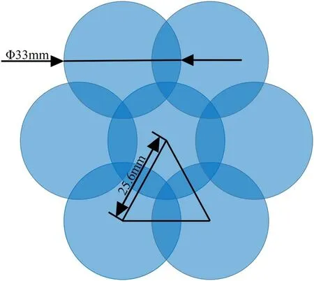
Figure 2.Schematic diagram of the overlapping multipositioner.The effective movement range of the end face of each positioner is a Φ33 mm circle,and the central distance between adjacent positioners is 25.6 mm.

This optical fiber positioning method has high positioning accuracy and positioning efficiency.The Sloan Digital Sky Survey (SDSS) telescope utilized the perforated positioning method in the early days,which required the installation hole to be made according to the star coordinates on the aluminum plate,and each optical fiber was inserted before observation, which was very inefficient in terms of positioning (Macktoobian et al.2019).Early on, the Subaru telescope employed the pendulum positioning method for the needle.This approach controls the piezoelectric actuator through a zigzag voltage pulse signal,tilting the mechanical structure of the fiber mounted to the target position, thereby completing fiber positioning.However, this positioning method brings about insufficient optical fiber light intake and light defocusing problems, and the positioning efficiency is not high enough.The new SDSS and Subaru projects choose to be similar to the LAMOST dual-rotation positioning method, which greatly improves the accuracy and efficiency of optical fiber positioning (Fisher et al.2012, 2014;Grossen et al.2020).The current Dark Energy Spectroscopic Instrument (DESI) telescope with 5000 fibers also adopts this optical fiber positioning method to achieve larger-scale optical fiber positioning(Leitner et al.2018;Poppett et al.2018;Zhang et al.2018; Fagrelius et al.2020).

1.2.Introduction to the Fiber Positioner Drive

The transmission structure of the central shaft is diagrammed in Figure 3.The central driving motor is connected to the motor interface plate.The motor interface plate is fixed on the fiber positioner with screws.The motor gear is fixed on the motor shaft with a locking nut and rotates with the motor shaft.The gear meshes with the internal gear,and the internal gear and the central shaft are fixed with set screws.The central rotary mechanism is driven by a stepper motor with a 1:1024 reducer through a two-stage spur gear to drive the hollow shaft to perform central rotation within the range of 0°–360° to realize the transmission of the central rotary shaft.The structure of the eccentric shaft drive is drawn in Figure 4.The eccentric driving motor is connected to the motor interface plate.The motor interface plate is fixed on the fiber positioner with screws.The motor gear is fixed on the motor shaft with a locking nut and rotates with the motor shaft.This gear meshes with the helical gear,the helical gear is tightly sleeved on the intermediate shaft and the other helical gear is tightly sleeved on the shaft to mesh with the eccentric helical gear.The locking nut fixes the helical gear on the eccentric rotary shaft to achieve transmission of the eccentric rotary shaft.The eccentric rotary mechanism is rotated by a stepper motor with a 1:16 reducer through a twostage single-tooth-multitooth helical gear reduction device for 0°–180° rotation to achieve the transmission of the eccentric rotary shaft.

The fiber positioner on LAMOST adopts an AM1020 stepper motor from the Faulhaber Group in Switzerland.When the center stepper motor operates with a minimum number of pulses, the minimum drive arc length is 3.31 μm.When the eccentric stepper motor runs with the minimum number of pulses, the minimum transmission arc length is 1.687 μm.Therefore,the central rotary shaft and the eccentric rotary shaft operate very precisely,and the theoretical positioning accuracy can reach the micron level.The operational accuracy of the overall fiber positioner can be guaranteed under open-loop operating conditions, and this will also provide the possibility of performing closed-loop control positioning on the optical fiber positioning system in the future.

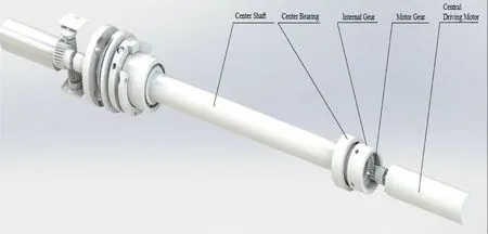
Figure 3.Structural diagram of the central shaft transmission.The central driving motor, through the motor gear and internal gear meshing process, realizes the transmission of the central rotary shaft.

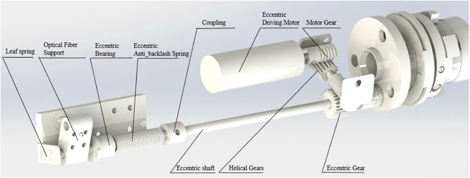
Figure 4.Structural diagram of the eccentric shaft transmission.The eccentric driving motor drives the eccentric rotary shaft through two-stage single-tooth and multitooth helical gears.

1.3.Diagnostic Method of the Operational Accuracy of the Fiber Positioner

The positioning accuracy of the fiber positioner directly affects the observation efficiency of LAMOST, and when the positioning accuracy of the fiber positioner is unacceptable, at first, the possibility of interference caused by adjacent positioners increases, and the positioner cannot effectively converge.Second, when the positioner installed in the focal plane of LAMOST receives light from celestial bodies,it cannot accurately reach the position required by the system instructions due to the unsatisfactory positioning accuracy of the positioner;thus, the observation target cannot be found.When the positioning error of the fiber positioner is greater than 40 μm,the observation target cannot accurately fall on the center of the fiber,and when the positioning error is greater than 100 μm,the fiber cannot be aimed at the astronomical target.To ensure the observation efficiency of LAMOST, we define fiber positioners with positioning errors greater than 40 μm as unqualified positioners during positioner maintenance.

Because the fiber positioner is composed of many complex parts, the failure rate of the positioner will increase with increasing use time after long-term operation.The frequent failures are divided into two types: central shaft failures and eccentric shaft failures.The faults of the central shaft include faults of the inner gear of the central shaft, looseness of the anti-backlash spring plate and the motor gear,and central shaft motor damage.Furthermore, the faults of the eccentric shaft include faults of the eccentric shaft anti-backlash spring plate,gear faults, loosening of the fixing screw of the optical fiber bracket and damage to the eccentric shaft motor (Gan et al.2007).When the above problems occur in the positioner, its stability and reliability decrease, and the observation accuracy decreases accordingly (Cheng et al.2018).

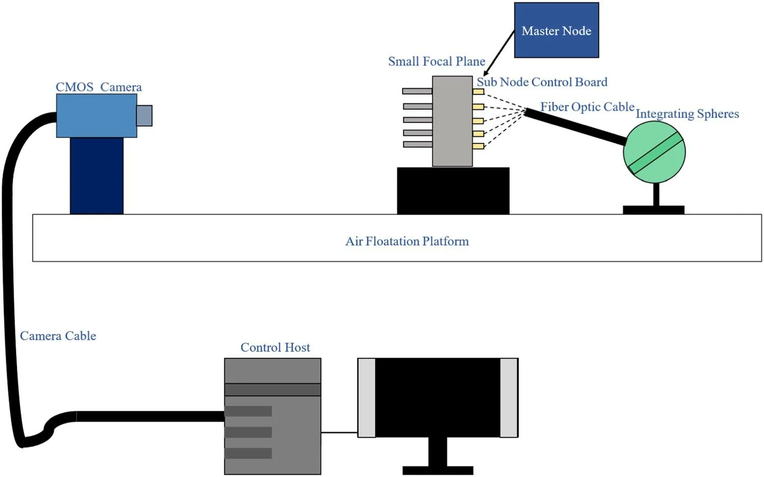
Figure 5.Fine run-in system of the fiber positioner.The system can achieve the control drive of the fiber positioner and the real-time measurement of the fiber position.

Therefore, once LAMOST operates normally for more than ten years,normal routine maintenance of the fiber positioner is required every summer, and the positioner is maintained and repaired to ensure its stability and reliability.At present,during the process of maintaining the positioner, for a positioner with unqualified accuracy, the cause of the positioner failure is analyzed through manual maintenance experience.Then, the corresponding positioner maintenance process is carried out according to the cause of the failure.However, in the stage of analyzing the cause of the positioner failure,it takes a long time to find the cause of the failure because the scope of the fault is not clear.This makes the positioner maintenance process take a long time and causes the maintenance efficiency to be low.

To solve this problem, a new fault analysis and detection method is proposed in this paper.Section 2 mainly describes,based on photogrammetry, how to obtain repeated positioning accuracy and open-loop calibration curve data of the optical fiber positioner.Furthermore, the operating characteristics of the fiber positioner are systematically analyzed to classify the observed faults.In Section 3, deep learning-based long shortterm memory (LSTM) model training is applied to achieve rapid classification and location of the fault cause of the optical fiber location positioner.In Section 4, the experiment and its results are summarized.

2.Fine Run-in Experiment of the Fiber Positioner

2.1.Fiber Positioner Running and System Precision

At present,the positioning accuracy of the fiber positioner is measured through a running and testing platform built in the laboratory.The specific composition of the running and testing platform is depicted in Figure 5.

The whole system consists of five main parts: the fiber positioner, a small focus panel, a control part, a measurement subsystem,and a light-guided fiber and light source.The small focus panel, the fiber positioner, and a complementary metaloxide-semiconductor(CMOS)camera are installed on the same air-floating platform.

Small focus panel:In this part,276 holes are processed on the focus panel in a honeycomb shape for the clamping positioner.As shown in Figure 6,a fiber positioner can be installed in each hole position,and the focal panel is perpendicular to the floating platform.

Control part: The control host controls the camera, and the main node controls the subnodes installed in the fiber positioner through wireless communication to make the positioner run.

Light-guided fiber and light source: The integrated sphere provides a uniform illuminating light source for the optical fiber.

Figure 6.Front view of the small focus panel.The figure shows 276 fiber positioners and reference fibers mounted on the small focus panel for detecting the positioning accuracy of the system positioner.

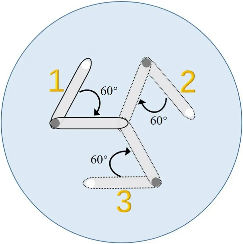
Figure 7.This figure illustrates the positions of the two shafts when the center shaft is running.When the central shaft runs,to accurately measure the motion trajectory of the central shaft drive, the eccentric shaft is spread out by 60°before running,and then the eccentric shaft is in a stationary state.The central shaft takes 300 pulses per step and 210 steps per round.Position 1 shows the initial positions of the two shafts,and positions 2 and 3 are the positions of the two axes passed during central shaft running.

Measurement subsystem:The camera used in the measurement system is the CV50000 CMOS sensor from COMSIS with 7920 ∗6004 4.6 μm 8T global shutter pixels.Moreover,the camera has a 3 mm full-frame optical format, and its temporal noise is 15.3 e-.In addition, the full well capacity of the camera is 16 000 e-, and the dynamic range is 60 dB.Finally, the lens has a typical(maximum)optical distortion of<0.08(0.20%)over its aperture,and the object-image relationship of the camera is 1 pixel,corresponding to 18.6 μm.We fully consider the impact of the distortion factors caused by the camera lenses on the measurements obtained in the experimental work.Before collecting the motion accuracy data of the fiber positioner, we perform camera calibration on the CMOS camera.The purpose of camera calibration is to solve the camera parameters, which include camera distortion parameters, and can effectively correct the distortion of the camera lens itself.This paper uses a polynomial calibration model to solve the camera parameters by relying on a calibration target.The calibration target is installed at the focal plane, and the CMOS camera parameters are solved using the polynomial calibration model to correct the distortion of the camera lens itself.Since the calibration target is in the same plane as the fiber-optic endpoint, the obtained camera parameters can accurately capture the motion accuracy data of the fiber positioner.The camera calibration process is carried out on a running and testing platform built in the laboratory environment of the University of Science and Technology of China.After the camera calibration process is completed, the CMOS camera captures the calibration target, and the residual distance between the actual coordinates and the theoretical coordinates is 4.6 μm.The CMOS camera has high measurement accuracy, satisfying the fiber positioning accuracy requirement of LAMOST.

At present, whether the positioning accuracy of the fiber positioner meets the preset requirements is determined through the repeated positioning accuracy and the open-loop calibration curve data, and the data are accurately run and obtained through the running and testing platform.

2.2.Fine Run-in and Experimental Process of the Fiber Positioner

When the fiber positioner is running, the central rotary axis and the eccentric rotary axis are separately measured.We rotate the central shaft from 0° to 360° as a round and turn the eccentric shaft from 0°to 180°as a round.In addition,we set a certain number of pause measurement points as index points in each round,return to the original position after reaching the full stroke,and then perform the next round of measurement.When setting the indexing points, the number of indexing points should not be too few to reflect the accuracy of the precise meshing of the gears.Such a value would not be able to describe the running status of the fiber positioner in detail.In addition, the value should not be set too high so that the detection time does not become too long.A total of 210 division points are selected to meet the above requirements.As visualized in Figures 7 and 8, when the central shaft and eccentric shaft run for one round, the running pulse of the stepper motor is 63,000, that is, 300 pulses per step.To improve the pixel coordinate accuracy of each index point,the measurement is repeated ten times for each index point.During the process of running, the CMOS camera captures the fiber position coordinates of each indexing point and records the obtained fiber coordinates in the control host.This improves the accuracy of the measurement data and reduces errors.We generally set the central axis of each batch of fiber positioners,and the eccentric axis runs and tests for five rounds each.Since the positioner is still in the running-in stage at the beginning,the running process and the following rounds of the positioner will be more stable.Therefore, in the calculation process, we usually select the data from the third to fifth rounds of the optical fiber to participate in the calculation for obtaining the repetition of the fiber positioner.The positioning accuracy and calibration curve data are obtained.The fiber positioner is driven by a permanent magnetic motor through a reducer and a gear meshing transmission, which has high transmission accuracy and can reach the micron level.The three-wheel measurement can effectively reflect the repeated positioning accuracy, and the collection of more measurement rounds increases the measurement time and decreases the efficiency of the motion data measurement process.In addition, it does not have a significant influence on the repeated evaluation of the positioning accuracy.Therefore, the three-wheel measurement data satisfy the requirements for the repeated evaluation of the positioning accuracy.

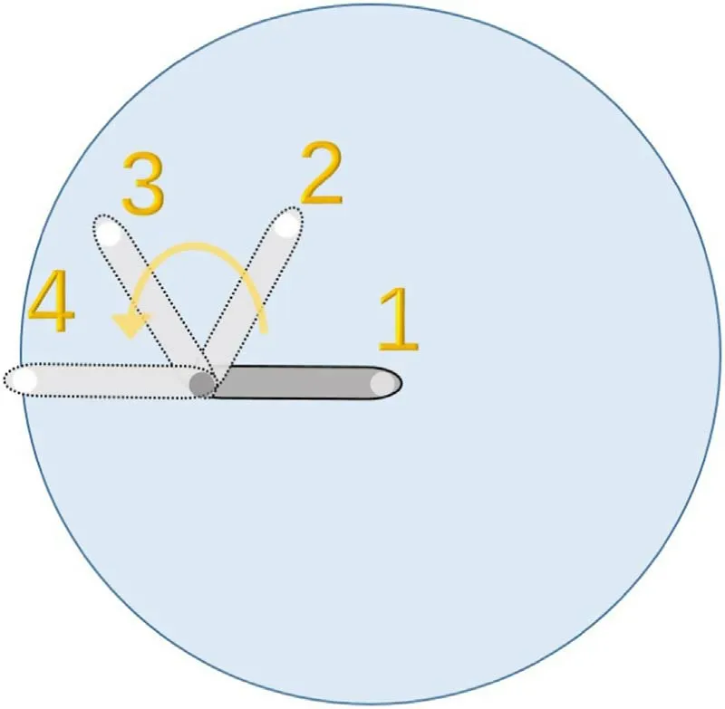
Figure 8.This figure illustrates the positions of the two shafts when the eccentric shaft is running.When the eccentric shaft runs,the central shaft is in a stationary state.The eccentric shaft takes 300 pulses per step, and each round takes 210 steps.Position 1 shows the initial positions of the two shafts, and positions 2, 3, and 4 are the positions of the eccentric shaft passed during the eccentric shaft running process.

2.2.1.Calculation of the Repeated Positioning Accuracy of the Fiber Positioner

The coordinates of each index point are measured ten times in a row in each round, and the average of the ten measurements is taken as the actual coordinate value of the index point for that round.After repeating this process for three rounds, the mean of the coordinates for each indexing point over the three rounds is obtained.The distance from the actual coordinate value of each division point in each round to the mean of the three rounds of division point coordinates is calculated.Finally, we calculate this distance for all the indexing points in these three rounds to determine the standard deviation (δ).Figure 9 displays the typical repeat positioning accuracy of the central axis and eccentric axis of the fiber positioner.The curve in each color represents the distance error between the actual value of the coordinates of each index point in the corresponding round and the average value of the actual coordinates of the index points in three rounds.

Figure 9.Typical repeat positioning accuracy diagram.The abscissa is the number of index point steps, and the ordinate is the distance from the actual coordinate value of each division point in each round to the mean of the three rounds of division point coordinates.The different colored curves represent the rounds corresponding to the run-in of the positioner.

Experimental data analysis:

The repeated positioning accuracy is based on multiple rounds of positioning at the same position of the fiber positioner.The stability and reliability of the fiber positioner can be qualitatively analyzed by plotting the distance between each indexing point and the actual average value of the coordinates of the three indexing points.Calculating the standard deviation can quantitatively provide a determination of whether its accuracy meets the imposed requirements.The LAMOST facility requires that the 3δ of the fiber positioner not exceed 40 μm to meet the requirements of the LAMOST observations regarding the positioning accuracy of the fiber positioner (Jin et al.2008).

In Figure 9, the standard deviation δ of the central axis distance of the fiber positioner is 1.6844 μm, the standard deviation δ of the eccentric axis distance is 1.9566 μm,and the 3δ between the central axis and the eccentric axis is far less than 40 μm.These results indicate that the fiber positioner has high repeated positioning accuracy and can fully meet the positioning requirements.

2.2.2.Fiber Positioner Calibration Curve Data Calculation

The average values of the last three rounds are taken as the data that participate in the calculation process,and the center of rotation and the two gyration radii of the central axis and the eccentric axis are fitted by the least-squares method.Afterward,the actual rotation angle of each step is calculated by using the parameters of the fiber positioner through the cosine theorem.

Least-squares fitting method:

We suppose that (x, y) are the coordinates of the center of rotation, r is the radius of rotation, and (xi, yi) are the coordinates of the ith division point.According to the definition of a circle,

where x and y are the horizontal and vertical coordinates of the rotation center, and xiand yiare the horizontal and vertical coordinates of the ith division point,respectively,while r is the radius of the rotation trajectory.

It can be deduced from Equation (1) that

We let

The following matrix can be obtained:

We find the coordinates of the center of rotation (x, y) and the radius of rotation r.

Actual step angle calculation:

Figure 10.Schematic diagram of the step angle calculation process for the central and eccentric axes.Each point in the figure represents the position of the fiber when the positioner stalls at the indexing point,the central shaft indexing point trajectory is circular and the eccentric shaft indexing point trajectory is semicircular.

We let the angle between the ith and the i+1th division point be θi; the lengths of the three sides of the triangle are la,lb, and lc.The three side lengths of la, lb, and lccan be calculated from the distance formula between two points in a plane.Finally, as shown in Figure 10, according to the cosine theorem, we obtain

where la, lb, and lcare the lengths of the sides of the triangle formed by the rotation center and the ith and i+1th division points, while θiis the angle between laand lb.

Experimental data analysis:

As seen in Figure 11,the theoretical step angle of each index point of the central axis is 1.72°, and the step angle of each index point of the eccentric axis is 0.86°.However, the actual calibration curves of the two axes are near their theoretical values.The fluctuation, i.e., the number of pulses, and the actual rotation angle are not simply linear.

2.3.Analysis of the Accuracy Error of the Fiber Positioner

Quantitatively, a fiber positioner with unqualified positioning accuracy has 3δ > 40 μm, and qualitatively, the repeated positioning accuracy curve and calibration curve fluctuate greatly.The failure cause of the unqualified positioner must be analyzed,and the common failure causes affecting the positioning accuracy of the positioner are divided into four types.

1.The assembly of the parts of the eccentric shaft transmission is loose.

The looseness of the assembly of the parts of the eccentric shaft transmission is divided into eccentric shaft anti-backlash spring looseness, the eccentric shaft gear looseness, and the looseness at the optical fiber bracket due to a set screw.Eccentric shaft gear looseness is the most common of these causes.The cause of the fault induces a backlash impact when the eccentric shaft gear is driven such that the eccentric shaft transmission is not synchronized, and the optical fiber transmission to the target point has a certain deviation.

Figure 11.Typical calibration curve.The abscissa is the number of index point steps,and the ordinate is the step angle between the indexing point of each step and the next indexing point.The different colored curves represent the rounds corresponding to the run-in of the positioner.

As affirmed in Figure 12, because the optical fiber transmission position has a certain deviation from the target point, the residual error of the optical fiber coordinate of each indexing point increases, and the oscillation amplitude of the step angle of the indexing point increases.

2.The eccentric shaft motor is damaged.

Figure 12.Case when the eccentric shaft gear of the fiber positioner is loose.The standard deviation of the eccentric shaft distance in three turns of the failure cause (δ) is 28.8509 μm.The step angle of each index point of the eccentric axis is between 0.°6 and 1.2°, and the theoretical step angle is 0.86°.

When the eccentric shaft motor is damaged, the eccentric shaft motor gear cannot be stably driven, the eccentric shaft cannot reach the exact required position when it is driven and the position of each round of optical fibers is not fixed.

As shown in Figure 13,due to jittering that occurs when the eccentric shaft is driven, the position coordinates of each indexing point are not fixed, and the residual error of each indexing point is large.Similarly, the step rotation angle of each indexing point in the calibration curve is also high.

3.The assembly of the parts of the central shaft transmission part is loose.

Figure 13.Case with damage to the eccentric shaft motor.The standard deviation of the eccentric shaft distance in three turns of the failure cause(δ)is 642.6237 μm.The step angle of each index point of the eccentric axis is between 0.°4 and 1.2°, and the theoretical step angle is 0.86°.

The looseness of the assembly of the parts of the central shaft transmission is caused by the looseness of the internal gear of the central shaft and the looseness of the anti-backlash spring of the central shaft.Among them, the looseness of the internal gear of the central shaft is the main cause.When the central shaft runs in harmony, the motor gear meshes with the internal gear, driving the internal gear to operate.Since the internal gear is not fixed with the central shaft,it cannot stably drive the central shaft to rotate, resulting in lost steps and a large error distance between the central shafts of different wheels.

As demonstrated in Figure 14,due to the loss of steps during the transmission of the central shaft, the position of the indexing point in each round will not be fixed,and the residual curve will fluctuate greatly.

4.The central axis motor is damaged.

If the motor of the central shaft is damaged,when the central shaft runs in harmony, the motor gear cannot be driven stably,resulting in a large shaking of the central shaft.Moreover, the position of each indexing point in each round is unstable.

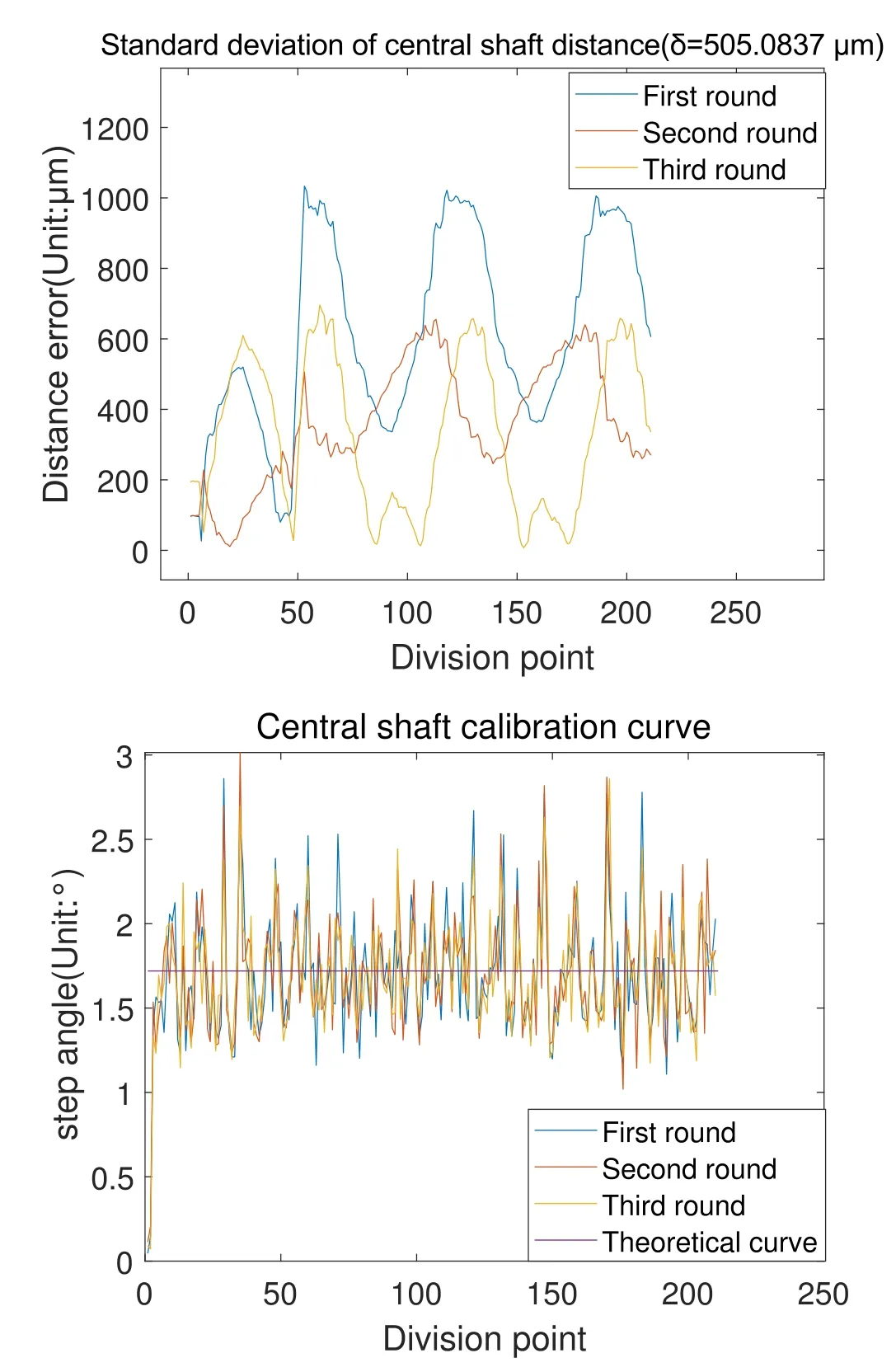
Figure 14.Looseness of the internal gear of the central shaft.The standard deviation of the eccentric shaft distance in three turns of the failure cause(δ)is 505.0837 μm.The step angle of each index point of the eccentric axis is between 1° and 3°, and the theoretical step angle is 1.72°.

As plotted in Figure 15, due to the severe jitter that occurs when the central shaft is driven, the position error of the same index point in each round will be very large, and the residual curve will fluctuate violently.Similarly,each index point in the calibration curve has a large fluctuation.

During the maintenance of the fiber positioner, we accumulate a large amount of data on the causes of positioner failures.We select 500 positioners that had undergone repairs and analyze the causes of their failures.Among the 392 positioners,the cause of failure is found to be the looseness of the assembly of the parts of the eccentric shaft transmission with a probability of 78.4%.For 257 positioners, the cause of failure is the looseness of the assembly of the parts of the central shaft transmission with a probability of 51.4%.For 21 positioners, the cause of failure is a damaged central shaft motor with a probability of 4.2%, while for 19 positioners, the cause is a damaged eccentric shaft motor with a probability of 3.8%.Since some fiber positioners may have several types of failure causes simultaneously, the sum of the probabilities of the failure causes may exceed 100%.

Figure 15.Damage to the central axis motor.The standard deviation of the eccentric shaft distance in three turns of the failure cause (δ) is 334.3656 μm.The step angle of each index point of the eccentric axis is between 0°and 2.5°,and the theoretical step angle is 1.72°.

These four types of fault causes can basically cover all operating conditions of the positioners.During the annual maintenance of a large number of fiber positioners, we classify the fault causes into four major categories.The main causes of failure are the looseness of the assembly of the parts of the central shaft transmission and the looseness of the assembly of the parts of the eccentric shaft transmission.In very few cases, the faults are caused by damaged central or eccentric shaft motors.

Therefore, we believe that these four types of fault causes can effectively cover the operational faults of the positioners.

3.Fault Diagnosis Based on an LSTM Deep Neural Network

3.1.Fault Diagnosis Method Selection

Existing fault diagnosis methods are mainly divided into traditional fault diagnosis algorithms and deep learning-based fault diagnosis algorithms.

Traditional fault diagnosis methods require manual feature extraction, feature selection, and fault classification.During feature extraction, time–frequency statistical feature analysis,the fast Fourier transform, the wavelet transform and time–frequency map analysis are often used to eliminate the influence of noise.To extract features that are suitable for fault classification, principal component analysis (Hu et al.2014), independent component analysis (Qu et al.2006),manifold learning, and other algorithms are chosen to screen useful features.Finally, by using a backpropagation neural network or support vector machine as the fault classifier(Feng& Zhang 2013), fault classification can be successfully achieved with good robustness.The traditional fault diagnosis algorithm,such as in the simple feature extraction method,has a wide range of applications, and can partially meet the imposed fault diagnosis recognition rate requirements by setting appropriate classifier parameters.However, the feature extraction process of traditional algorithms relies on manual extraction and expert knowledge in the field, and the generalization ability of the resulting model is not sufficiently robust.The above traditional methods have difficulty satisfying the fault diagnosis requirements of fiber positioners.

In contrast, fault diagnosis algorithms based on deep learning have also begun to emerge with the development of deep learning theory.Their strong robustness and extremely high accuracy bring new ideas to the field of fault diagnosis.Such an approach can automatically extract features from data without relying on the prior knowledge of experts and finally achieve fault classification, effectively improving fault diagnosis in terms of accuracy and efficiency.Based on the unique advantages of deep learning in automatic feature extraction and recognition, deep learning is selected in this paper for diagnosing the faults of fiber positioners whose positioning accuracies do not meet the set requirements.

3.2.Data Analysis and Model Selection

Most of the existing fault diagnosis algorithms based on deep learning utilize vibration data for analysis.However, for the LAMOST fiber positioner, due to its complex mechanical structure, these methods are not suitable for fault analysis through raw vibration signals.In this paper, through precision running and experiments involving the fiber positioner, four sets of positioner parameters are obtained: the repeated positioning accuracy of the central axis, the calibration curve of the central axis, the repeated positioning accuracy of the eccentric axis and the calibration curve data of the eccentric axis.These parameters can correspond one-to-one with the characteristics of positioner failures.Moreover, each group of data contains time series data,and the data are one-dimensional with strong contextual correspondence.Regarding the onedimensional data, a one-dimensional convolutional neural network (CNN) can extract their features very well, but a one-dimensional CNN has no memory ability and will waste the time features of the data (Qu et al.2018).In contrast, a recurrent neural network (RNN) can achieve time memory ability, but the traditional RNN model implements the backpropagation through time(BPTT)method during training(Zhu et al.2022).When the given time series is long, the residual error that needs to be returned decreases exponentially.As a result, the network weights are updated slowly, and the model does not have a long-term memory capability.The LSTM model relies on a special hidden layer cell structure (Kaplan et al.2021), as shown in Figure 16.The input of each neuron not only has the training data input at the current moment but also the state input of the neuron at the previous moment.This provides the LSTM model with a powerful context memory ability and enables it to solve the problems of gradient disappearance and gradient explosion.Thus, it has a good ability to extract features from sequence data.It has been widely used in deep learning tasks such as text learning and speech signal processing (Song et al.2021).Therefore, the LSTM network is selected in this paper to extract fault features and build a fault classification model based on the given data and the accuracy metric.We classify the fault causes by making the error curves of different fault positioners correspond to different fault types.When using the LSTM network,we also employ these error curves as training data for the network.

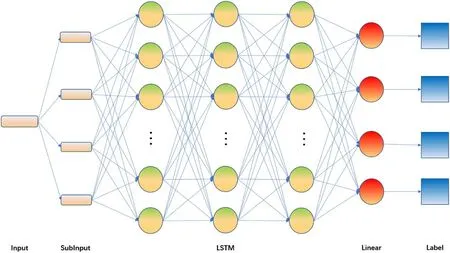
Figure 17.LAMOST double-turn positioner fault detection framework based on the LSTM model.The input layer represents 4 ∗210-dimensional input data,and the input data are divided into four sets of 210-dimensional input data according to the central axis and eccentric axis.LSTM is a concrete internal network model that consists of three layers with 500 neural nodes in each layer.The linear layer linearly maps the 500-dimensional data acquired by the LSTM to four dimensions.Finally, in the linear layer, the output results and labels are compared by the cross-entropy function to judge the model training situation and determine the optimization direction of the model parameters.

Figure 16(a) is a schematic diagram of the LSTM forward propagation model.xt−1, xt, and xt+1represent the data of the previous moment, the current moment, and the next moment,respectively.A is the neuron that needs to be trained in the LSTM model.ht−1,ht,and ht+1represent the states of neurons at the previous moment, the current moment, and the next moment, respectively.Figure 16(b) shows the internal structures of neurons.When neuron A is trained, three parts of the data are input: ht−1, the state of the neuron at the previous moment; Ct−1, the output of the neuron at the previous moment;and xt,the input data at the current moment.The forget gate inside neuron A, ft, the update gate it, and the state gate otare processed according to the input data in Equations (7)–(9), respectively.σ is the sigmoid nonlinear activation function that is often used in deep learning networks,as shown in Equation (6).Wf, Wi, and Woare the weight data for the various parts.bf,bi,and boare the offsets of the different parts.After completing further processing, such as the steps in Equations (10) and (11), the output Ctat the current moment and the state htof neuron A are obtained.The model designed in this paper is trained for multiple epochs, and each neuron obtains appropriate weight data, which can successfully classify the failure data.

σ is the nonlinear sigmoid activation function that is often used in deep learning networks.

ftis the forgetting gate inside neuron A.itis the update gate inside neuron A.otis the state gate inside neuron A.Wf, Wt,and Woare the weight data for each part.bf, bi, and boare the offsets of the different parts.

Ctis output of neuron A at the current moment.htis state of neuron A at the current moment.

3.3.Concrete Model Construction

As displayed in Figure 17, in the designed detection framework, the positioner running and accuracy data are 4 ∗210-dimensional data, which we send to the LSTM model for data feature extraction.The time length of each group of data is 210,and the number of features in each moment of data is four.The LSTM model has a total of three hidden layers, and each hidden layer has 500 nodes.After the feature extraction process of the LSTM, a 500-dimensional high-dimensional feature vector is output, the data features are reduced to four dimensions through the fully connected layer, and the maximum direction of the four-dimensional vector is the predicted feature direction.For the prediction result, we use cross-entropy to calculate its loss function,calculate the model gradient through the BPTT gradient backpropagation algorithm, use the ADAM optimization algorithm to update the model parameters, and finally obtain a converged model.

3.4.Data Preparation and Preprocessing

After viewing a long-term maintenance task of the LAMOST fiber positioner, we find that the failures of the positioner can be classified into four categories:eccentric shaft motor damage,eccentric shaft part looseness, central shaft motor damage, and central shaft part looseness.

Therefore,we use four double-turn positioners that break the central shaft and eccentric shaft according to four kinds of faults; that is, one positioner corresponds to one kind of fault.Afterward, the positioner is inserted into the test platform for calibration and running, and 2000 rounds of data are obtained for each fault.As shown in Table 1, we divide the data into a training set and a test set according to a ratio of 4:1; that is,each fault training set has a total of 1600 pieces of data, and each fault test set has a total of 400 pieces of data.Each fault data label is set to 0, 1, 2, or 3.

Figure 18.Loss function and accuracy changes observed during training.The result of each training epoch is evaluated using the cross-entropy function to calculate the loss rate,as shown in(a).As the number of training rounds increases,the loss rate decreases,and the model finally achieves convergence.The accuracy rate is the amount of data correctly classified after each round of training divided by the total amount of training data, as displayed in (b), and the accuracy rate continues to improve as the number of training rounds increases.

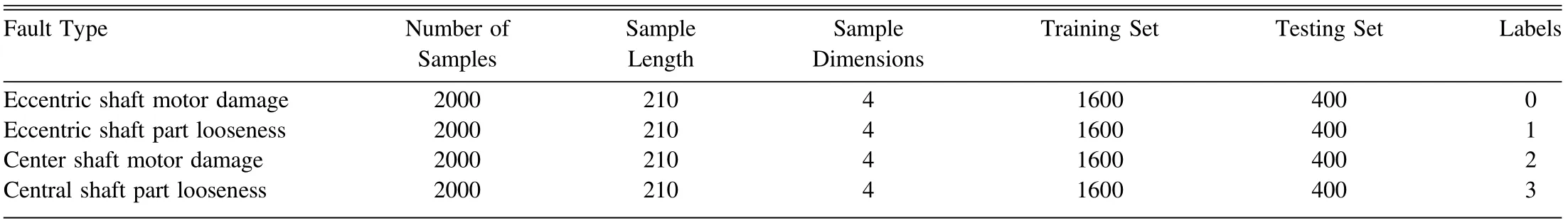
Table 1Composition of the Training Samples

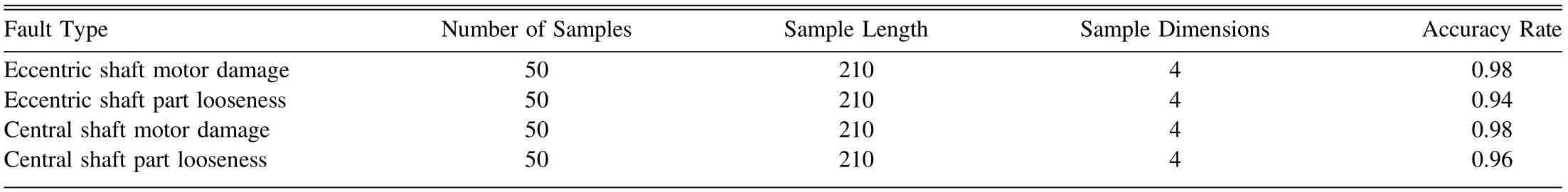
Table 2Actual Data Validation Results

3.5.Training Results

In this paper,the number of training rounds is set to 100,the training data are randomly scrambled and each batch has 500 pieces of data for training.After 100 rounds of training, the model converges, the accuracy rate achieved on the test set exceeds 98%,and the accuracy rate achieved on the validation set exceeds 97%.The model has a good fault data identification ability.Figure 18 shows the changes in the accuracy rate and loss function that occur during the training process.The loss function of the model decreases as the number of training rounds increases,and the accuracy rate gradually exceeds 98%as the number of training rounds increases.Figure 19 features the visual classification results of the final trained model for the failure data.The LSTM model can accurately distinguish the data of the four types of faults,and the features of each type of fault can be accurately extracted, indicating that the trained model has good feature extraction capabilities.

3.6.Validation Experiments with Actual Data

During a dual-turn positioner precision run and operation conducted at the LAMOST site, we obtain a large amount of failure data.We select 200 pieces of fault data and input them into our fault diagnosis model to verify whether the generalization ability of the model is effective.

As shown in Table 2,it is verified that the constructed model can successfully diagnose the fault data of the LAMOST field positioner.In follow-up maintenance tasks,we will continue to update more fault models in the maintenance task module to achieve rapid fault type diagnosis.Moreover, the maintenance task generates considerable positioner failure data every year,which we can use to further optimize the model and enhance the generalization ability of the model.

4.Conclusions

In this paper,a method for obtaining the repeated positioning accuracy and calibration curve data of a fiber positioner through photogrammetry and systematically analyzing the causes of the positioner failures that do not meet the imposed requirements during the operation of the LAMOST is proposed.The deep learning model classifies the positioner failure data and can accurately distinguish the causes of positioner failures.An efficient method for performing positioner fault classification and diagnosis is explored to greatly reduce labor and time costs and accumulate a large amount of reliable data for the design,processing, and assembly of subsequent positioners.This method can effectively reduce the probability of interference from adjacent fiber positioners, improve the convergence speed of positioners, and improve the observation efficiency of LAMOST.The maintenance and design optimization of this type of fiber positioner with a double-turn gear transmission system will be of general significance in the future,and a similar positioner fault diagnosis process will be carried out during the operation of fiber-optic positioners with double-turn mechanical structures, such as DESI and SDSS-V, and will serve as a reference.The sizes of fiber positioners in the future will be less than 10 mm.Because the transmission chain of such a positioner is simpler and more efficient, its structure will be pushed to the limit of conventional processing, and the failure rate will increase.The process of tracking and analyzing the causes of the positioning accuracy errors induced during operation is an essential analysis tool for the implementation of the next generation of miniaturized fiber positioners.

At present, the number of samples for training a deep learning-based LSTM model is not sufficient.In subsequent practical applications, it will be necessary to continue to accumulate a large amount of data to improve the generalization ability of the LSTM model.The next research direction will mainly be based on the large amount of positioner data obtained in practical applications that do not meet the imposed precision requirements, and we will divide fixed optical fiber positioner faults into more detailed failure causes to provide data support for the subsequent design, manufacture, and processing of fiber positioners.

Acknowledgments

Funding for the research was provided by Cui Xiangqun’s Academician Studio.The Guoshoujing Telescope [the Large Sky Area Multi-Object Fiber Spectroscopic Telescope(LAMOST)] is a National Major Scientific Project built by the Chinese Academy of Sciences.Funding for the project has been provided by the National Development and Reform Commission.LAMOST is operated and managed by the National Astronomical Observatories, Chinese Academy of Sciences.

Data Availability

The data underlying this article will be shared upon reasonable request to the corresponding author.

ORCID iDs

Zengxiang Zhou https://orcid.org/0000-0002-3050-5822