Detection of Pulsation and Additional Components in Eclipsing Binary RS Sct

A.Abedi and K.Y.Roobiat

1 Department of Physics, Faculty of Sciences, University of Birjand, Birjand, Iran; aabedi@birjand.ac.ir 2 Dr.Mojtahedi Observatory, University of Birjand, Birjand, Iran Received 2023 July 21; revised 2023 August 29; accepted 2023 September 27; published 2023 November 15

Abstract The eclipsing binary star RS Sct is a semi-detached system of the β Lyrae type.This system was photometered for six nights in 2019 August, and 2020 June and August.The light and radial velocity curves were simultaneously analyzed to obtain the absolute physical and orbital parameters of the system, and the system geometry was determined.In this system,the primary component has filled its inner Roche lobe and the secondary component is close to filling it.Moreover, the change in the orbital period of this system was investigated.The presence of the third or fourth components and the mass transfer between the two components affect the orbital period of the system.In addition, the pulsation of the primary component was detected.Also, several frequencies with high signal-to-noise ratios were identified.According to the position of the primary component in the H-R diagram and the value of the obtained frequencies, this component is likely a delta-Scuti pulsator.

Key words: (stars:) binaries: eclipsing – stars: individual (RS Sct) – methods: data analysis – techniques:photometric

1.Introduction

Based on recent findings, examples of pulsating stars can be seen almost throughout the H-R diagram (Aerts et al.2010).Asteroseismic studies have made significant progress with the initiation of projects such as CoRot,Kepler and recently TESS,as well as the provision of continuous and accurate light curves by these telescopes.These studies play an important role in obtaining the radius of the stars,and from this point of view,it can be very effective in determining the physical parameters of the stars.Binaries, like pulsators, exist in all parts of the Hertzsprung–Russell diagram (H-R) diagram, so most stars are present in binary or multiple systems(Duchene&Kraus 2013).If a binary eclipsing system is also of the two-line spectroscopic type, it is possible to directly determine the dynamic mass of the stars in these systems (Stebbins 1911).Therefore, when one or both components in a binary system are pulsating,the synergy created in these systems allows determining the physical parameters of the stars with high accuracy, and thus, in such systems it is possible to carefully examine and test the transformations and structure of the stars using a theoretical basis (Murphy 2018).

The eclipsing binary RS Sct (BD+40 442) was first discovered in 1907 by Pickering (Pickering 1907), and the first light curve of the system was presented visually in 1910 by Ichinohe (1910).The first light curve analysis for this system was done in 1913 by Shapley based on the photometric observations of Weil and Bakker (Shapley 1913).In 1916,Zinner raised the possibility that the orbital period of this system is variable(Zinner 1915).In 1936 and 1949,Piotrovsky studied the O −C curve of the minimum times of this system.He concluded that the data dispersion in this curve is more than what can be attributed to observational errors, so the orbital period of the system is most likely variable (Piotrowski 1936,1949).For the first time, Buckley performed the photometry of the RS Sct system by a photometer in 1980 and presented the light curve of this system using the Johnson-Cousins BVRI filters (Buckley 1980).Then, in 1984, Buckley analyzed these light curves in “detached” mode and reported the orbital and relative parameters of RS Sct.However,Buckley stated that due to the low quality of the data,it is not possible to comment with certainty on whether this system is “detached” or “semidetached,” and the solutions tended toward a semi-detached system(Buckley 1984).The radial velocity curve of this system was presented by King and Hilditch in 1984 (King & Hilditch 1984).These authors found that both components of the system have filled a significant part of their lobes while each of them has a temperature associated with the main sequence.Therefore,the two components have no temperature interaction with each other.In 1992,Cook studied the eclipse minimum times of this system and predicted the existence of a third component with a period of approximately 29 yr.He reported extreme and strange light changes, leading to the variation of the primary eclipse depth up to about 0.5 mag (Cook 1992).Investigations show that the simultaneous analysis of light and radial velocity curves of this system has not been performed.

2.Photometry and Data Reduction

The photometry of this system was carried out for two nights in 2019 August and four nights in 2020 June and August at the Dr.Mojtahedi Observatory of the University of Birjand using the V and R Johnson-Cousins filters.A 14 inch Schmidt–Cassegrain telescope equipped with an SBIG ST-7 CCD was used for the photometry of the system.During the photometry,the Maxim DL software was utilized to control and communicate with the CCD camera.The following linear ephemeris (Equation (1)) was used to calculate the system phase (Buckley 1984)

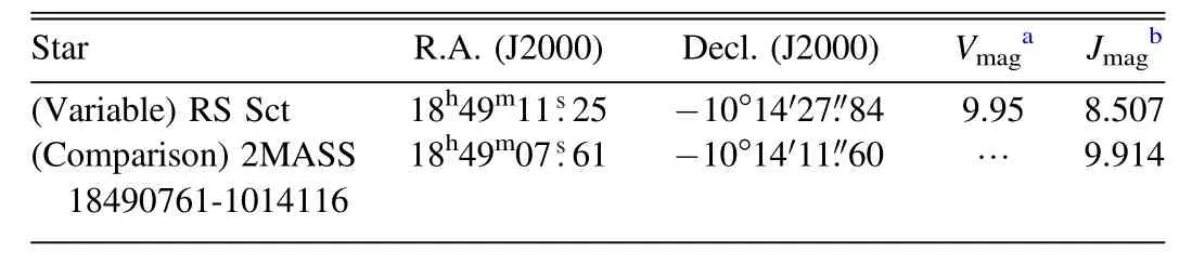
Table 1 Characteristics of the Variable and Comparison Stars

During the photometric process,the star 2MASS 18490761-1014116 was considered the comparison star.The characteristics of this star and the variable star are presented in Table 1.During the six nights of observing this system, 1828 images were obtained in the V filter and 1794 in the R filter.The image processing and data reduction were performed by the IRIS software.In these processes, we used the aperture photometry method.Effects of dark, bias, and flat images were applied to the astronomical images, and we found no zero-point shift between the nights.Figure 1 shows the light curves obtained in both V and R filters after normalizing to 1 at phase 0.25.The quality of the data in different nights is almost the same and there is no significant difference.Consequently,data dispersion can be due to the low accuracy of the used observational instrument (telescope and CCD) and other error-producing factors.In Figure 1, no special behavior can be seen in the residuals because the curve is drawn in terms of orbital phase,so the data related to different nights with time intervals are overlapped;however,if the residuals are plotted against time,a periodic behavior can be observed (see Section 5).

3.Light Curve Analysis

The PHOEBE Legacy program (Prsa & Zwitter 2005) was applied to analyze the light curves and determine the physical and geometrical parameters of the binary star RS Sct.First, the light curves of the system were analyzed in the “detached”mode.The “semi-detached” mode was used to analyze the system after we could not find a good match between the simulated light curve and the observational data in detached mode.In the detached mode, after running the program several times and leaving the parameters free to find a better fit between the observed data and the simulated curve, one of the components fills its inner Roche lobe and the system goes fromthe detached mode to the semi-detached mode.Therefore,if we limit ourselves to work in detached mode,no stable solution will be found for the system, and the value of Σ(O −C)2will be large.Investigations showed that the primary star in this system is non-spherical and has filled its inner Roche lobe.Based on the information in various catalogs, the temperature of the primary component is predicted to be between 6000 and 7200 K(Buckley 1984;Avvakumova et al.2013;Brown et al.2018).In the present study, the temperature of the primary component is chosen to be 7000 K.Moreover, the initial value of the secondary to primary mass ratio,q,was chosen as 0.6 based on the radial velocity curve presented by King & Hilditch (1984).According to the temperature of the primary component(T1<7200 K), the values of A1=A2=0.5 (Rucinski 1969)and g1=g2=0.32 (Lucy 1967) were used as fixed parameters for the bolometric reflection coefficients and gravitational darkening, respectively.Limb-darkening coefficients were automatically calculated by the software based on van-Hamme tables (van Hamme 1993) and using the logarithmic law.

Table 2 The Physical and Orbital Parameters of RS Sct Obtained from the Simultaneous Analysis of the Light Curves in the R and V Filters and the Radial Velocity Curve by the PHOEBE Program Along with the Results Obtained by Others

Finally,photometric data were analyzed simultaneously with radial velocity data (King & Hilditch 1984).In Table 2, the results of this research are compared with the results obtained by Buckley (1984).In this table, i is the orbital inclination,Vcomis the radial velocity of the center of mass of the system,Ω is the surface potential of the components, L is the luminosity of the component and r is the relative radius of the star.The synthesized light curves in the V and R filters are displayed in Figure 1, and the generated radial velocity curves are depicted in Figure 2.Figure 3 illustrates the three-dimensional (3D)structure of the RS Sct system at phase 0.75.

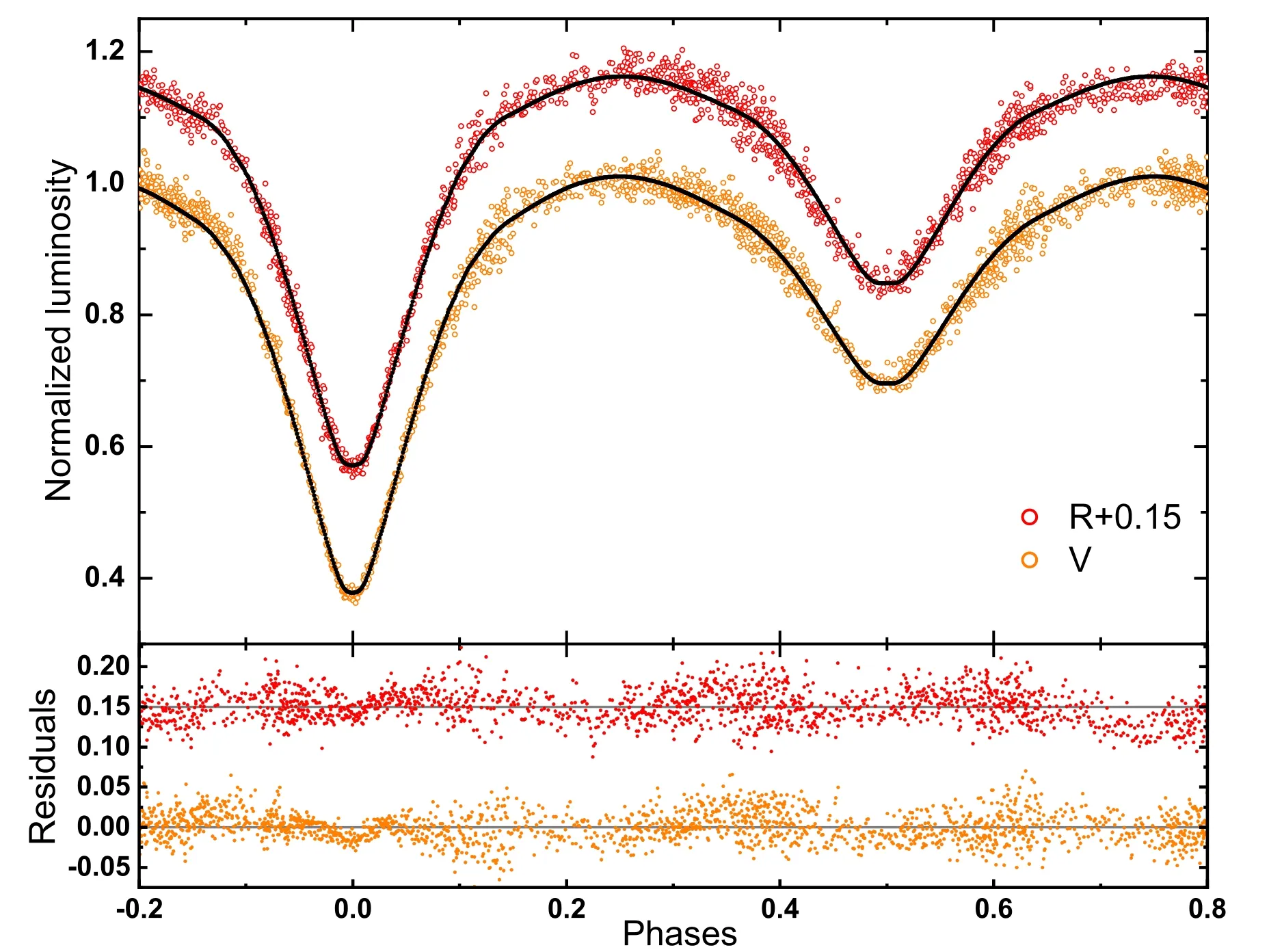
Figure 1.Light curves obtained for RS Sct in V and R filters.The points represent the observational data and the solid lines signify the simulated curves.The residuals are plotted in the bottom box.

Based on the radial velocity curve produced in the simultaneous analysis of the photometric and radial velocity data, the values of K1and K2were 115.24±5.2 km s−1and 189.73±9.8 km s−1, respectively.By using these values and the parameters reported in Table 2, the absolute parameters of the binary components of RS Sct were calculated.These parameters along with the values reported by Dryomova et al.(2005) are presented in Table 3.

With the help of the absolute physical parameters of the components of RS Sct and the use of the H-R diagram, the evolutionary status of the stars in this system was investigated.In Figure 4, in addition to the position of the components of this system, the positions of the components of several semidetached binaries(extracted from Malkov 2020)are presented.As seen in this figure, the primary component of RS Sct is located near the terminal age main sequence(TAMS)line,and the secondary component is above the main sequence.

In addition to the H-R diagram, the density–color index diagram can be used to check the evolutionary status of stars (Mochnacki 1981, 1984, 1985).The B −V color indices for the primary and secondary components of this binary system were obtained by referencing the tables in Worthey &Lee (2011) as 0.327(20) and 0.710(20), respectively.When using these tables, we assume that the two stars in the binary system do not affect each other, so they behave similarly to two single stars with the same chemical composition as the Sun.

Figure 5 shows the positions of the components of this system in the density–color index diagram.For comparison,the positions of the sample components,which have been obtained with a similar method in Malkov (2020), are also presented in this diagram.The positions of the components in this diagram are in agreement with the results obtained from the H-R diagram.Accordingly,the primary component of the system is close to the TAMS and the secondary component is outside the main sequence.

In 2006, based on a statistical analysis, Eker et al.obtained critical orbital angular momenta for contact binary systems based on the following equation (Eker et al.2006),

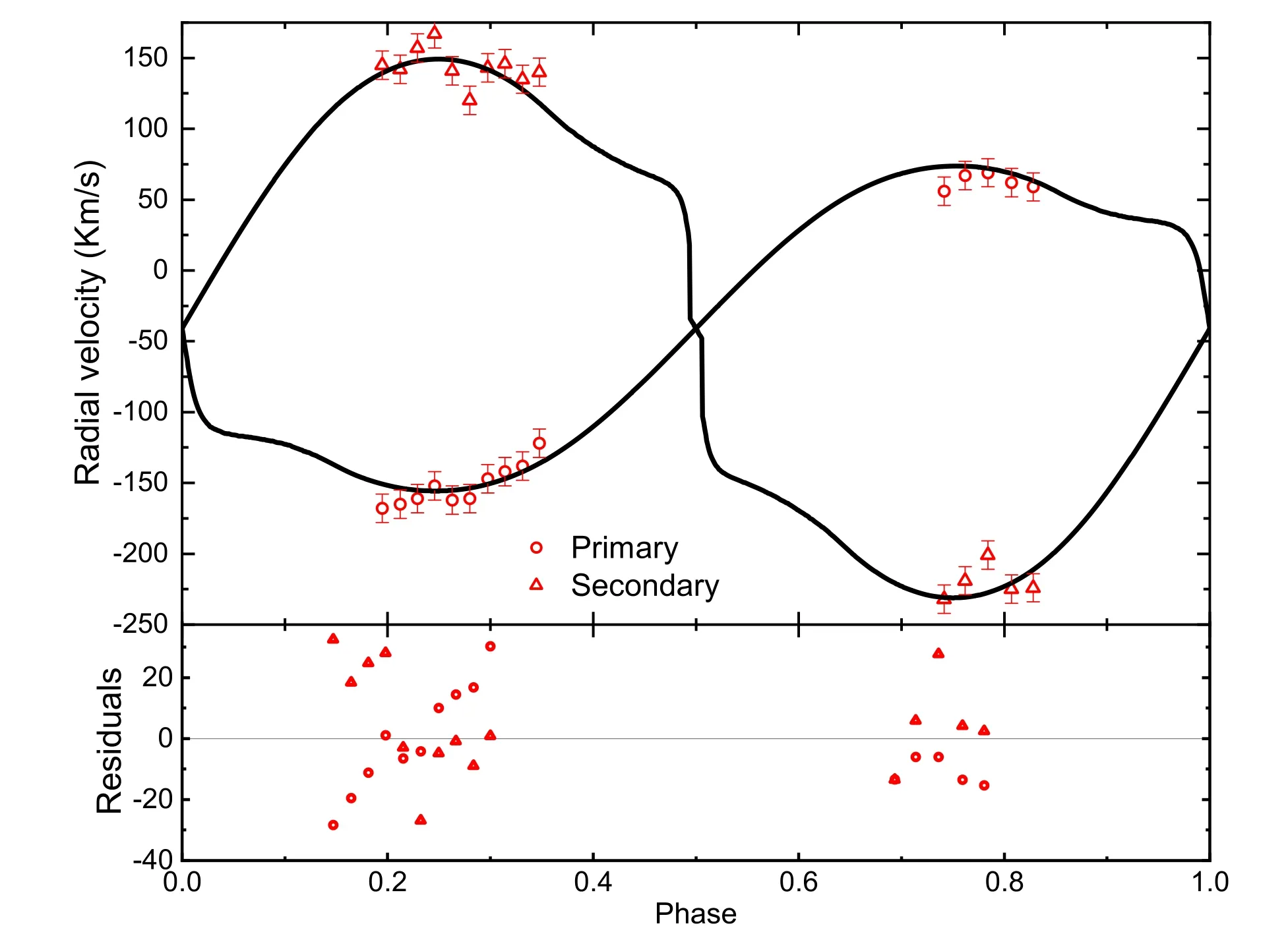
Figure 2.Radial velocity curves obtained for the RS Sct system.Points correspond to data reported in King & Hilditch (1984) and solid lines represent simulated curves.The residuals are plotted in the bottom box.

Figure 3.3D structure of RS Sct at phase 0.75.

Figure 4.The positions of the components of RS Sct in the H-R diagram.The positions of the components of several semi-detached binary systems are extracted from Malkov (2020) and plotted for comparison.Moreover, the zero age main sequence (ZAMS) and TAMS lines were obtained using MESA-Web (http://mesa-web.asu.edu).

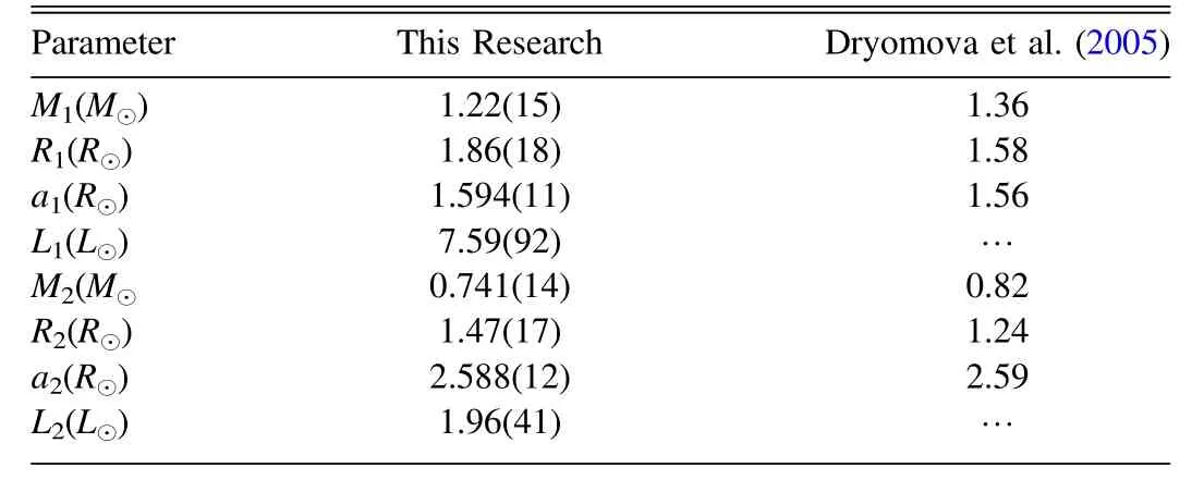
Table 3 Absolute Parameters of RS Sct and the Results Obtained by Others

In this equation, M is the total mass of the primary and secondary components of the system in terms of the Sunʼs mass.If the orbital angular momentum of the system is less than this critical value, the system is in contact, but otherwise,the system is semi-detached or detached.The magnitude of the orbital angular momentum for RS Sct is obtained using the following equation (Hu et al.2018)

The position of this system is marked in the plot of orbital angular momentum versus total mass in Figure 6.As can be seen in this figure,RS Sct is located near and above the critical momentum line, so the non-spherical geometry of components and semi-detached structure are most probable for this system.

4.Investigating Orbital Period

During the observation of the RS Sct binary system, four primary and two secondary minimum times were identified.To extract these minimum times, the method of Kwee & van Woerden (1956) was used; these minimum times are listed in Table 4.

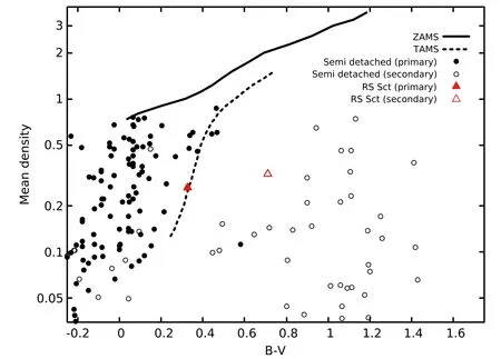
Figure 5.The positions of the components of RS Sct in the density–color index diagram.The positions of the components of several semi-detached binary systems are extracted from Malkov (2020) and plotted for comparison.Additionally, ZAMS and TAMS lines are taken from Figure 4 of Mochnacki (1981).

All the minimum times reported for this system were collected from the AAVSO and O −C gateway databases.After removing overlaps, the O −C curve of this system was plotted using these minimum times plus the minimum times that are listed in Table 4.To investigate the changes in the orbital period of this system,we had 318 minimum times from which 261 were related to visual data,17 to photographic data,and 40 to photoelectric and CCD data.Due to the lower accuracy of visual data and photography compared to photoelectric and CCD data, different weights were assigned to the data types in the analysis of the O −C curve.These weights were 1,3 and 10 for visual data,photographic data and photoelectric/CCD data, respectively.This method of weighting the observational data is also common in the literature; for example,see Zasche et al.(2008),Hanna&Amin(2013),Ulas et al.(2020).Moreover, the linear ephemeris given in Equation (1) was used to calculate the epoch and O −C.In Figure 7,the O −C curve of the minima of the eclipsing binary RS Sct can be seen.

In semi-detached and contact systems, mass transfer is one of the main mechanisms of orbital period changes, which can be checked by fitting a second-order function to the O −C curve.Therefore, a second-order function was fitted to the O −C curve of RS Sct and its coefficients were obtained using the least squares method.Based on the obtained coefficients for this second order function and following the Kalimeris method(Kalimeris et al.1994),the new linear ephemeris of this system was calculated as follows

Considering the mass transfer effect, the nonlinear ephemeris of the system can be written as

The orbital period reduction rate of the system was also calculated as follows (Hilditch 2001)

According to the semi-detached geometry and dimensions of the stars in this system, the mass transfer between the components is probably conserved.With this assumption, the mass transfer rate is as follows (Hilditch 2001)

In Figure 7, the second-order function is fitted to the O −C curve of RS Sct.After subtracting this second-order function from the O −C curve, a periodic behavior can be seen in the residuals.

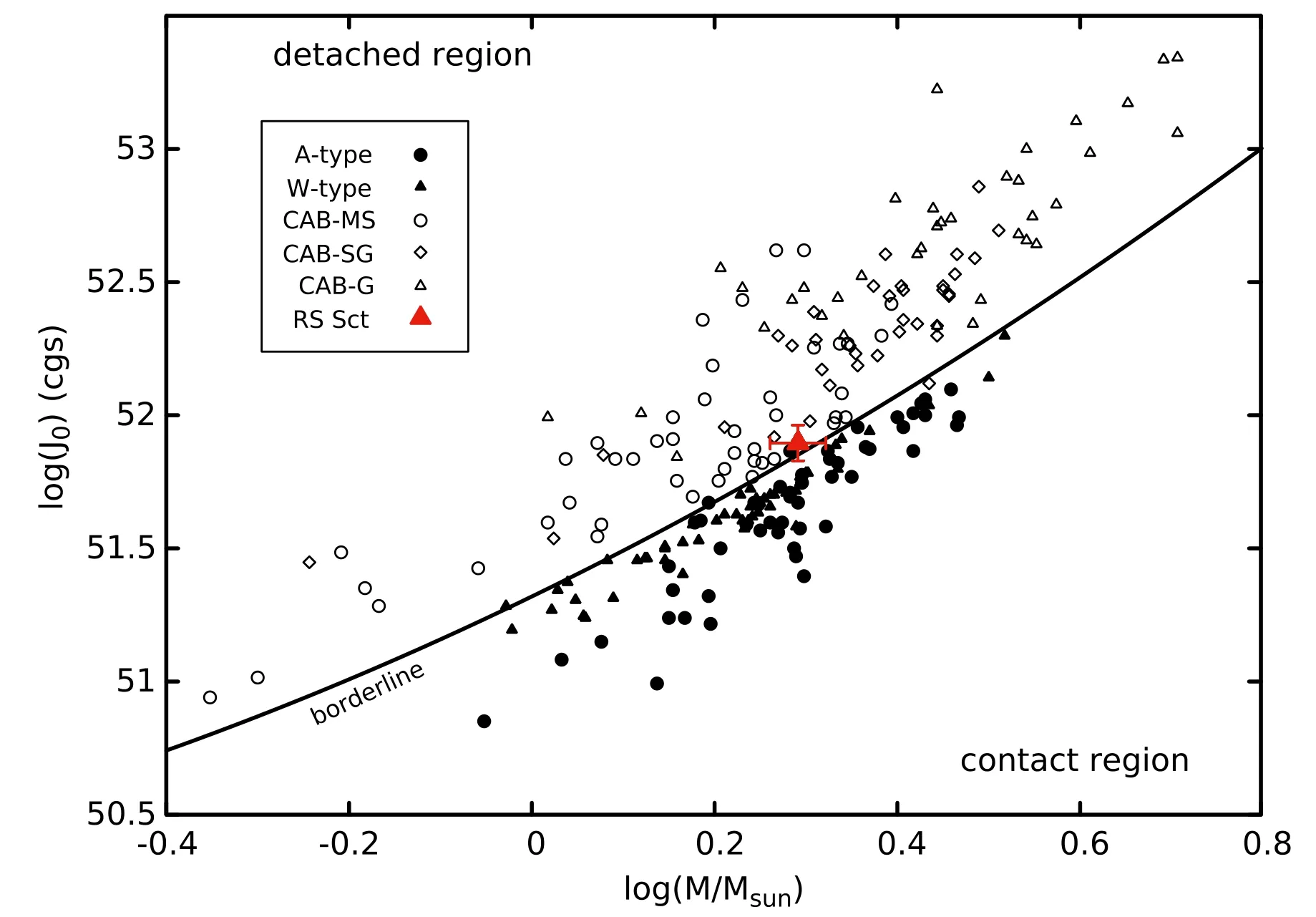
Figure 6.Position of RS Sct in the plot of orbital angular momentum vs.total mass.Examples of binary systems are extracted from Eker et al.(2006).CAB indicates systems with an active chromosphere while G, SG and MS indicate systems that contain at least one giant, one subgiant and two-component systems in the main sequence, respectively.

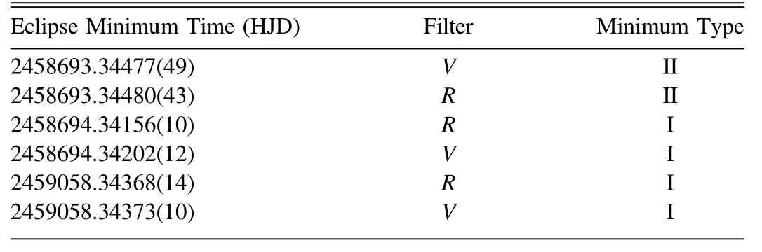
Table 4 The Minimum Times Obtained for RS Sct in this Research

These periodic changes can be attributed to the light-time effect caused by one or more other components in this system.To investigate the light-time effect in the O −C curve, the following relationship was used (Irwin 1959)

where k, e, ω and ν are the amplitude of O −C changes,eccentricity, longitude of periastron, and true anomaly of the third or fourth body, respectively.To find the initial value of the orbital period of this additional component(or components)in RS Sct,we employed the Period04 program(Lenz&Breger 2005).However, to fit Equation (8) to the residuals of the O −C curve, the orbital period was taken as a free parameter.The best fit to the residuals of the O −C curve was obtained by considering the two light-time effects corresponding to the existence of the possible third and fourth components in this system.The results of this analysis are given in Table 5 and Figure 7 to show the final fitting and final residuals.By adding a fourth object to the system, the value of χ2is reduced from 0.02555 to 0.02075.Also, to be absolutely sure, we applied a statistical F-test for comparing one- and two-additionalcomponent models.For the model including the mass transfer and light-time effect of the third object, the value ofwas obtained to be 1.8769, and there were eight free parameters in the model.Therefore, this model is acceptable by up to 5% error.For the model including mass transfer and light-time effects of the third and fourth bodies with 13 free parameters, the value ofwas obtained to be 0.1574, so this model is acceptable by up to 0.1%error.Accordingly,by examining this statistical test,it is clear that adding a fourth body to the model has improved the results.After removing the effects of the second-order function and the two light-time effects associated with the third and fourth components,the final residuals are randomly distributed around the zero line with no systematic behavior.Therefore, it seems that there is almost no other factor that causes a change in the orbital period of the system.

Figure 7.O −C curve of RS Sct.Dashed line:second-order function fitted to the data.Blue line:the sum of the second-order function and the light-time effect of the third object.Red line:the final fitted curve including the sum of mass transfer and light-time effects related to the third and fourth components.The final residuals are plotted in the bottom box.

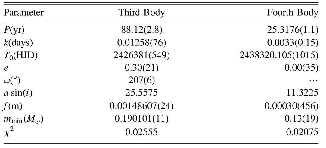
Table 5 Physical and Geometric Parameters Obtained for the Third and Fourth Components of RS Sct

5.Checking the Presence of Pulsation in the Components

To investigate the presence of pulsations in the components of RS Sct, we need to obtain the residuals of the light curve between the model and observations.These residuals can be seen in Figures 8 and 9 for V and R filters, respectively.To better show the behavior of the residuals in terms of time, the horizontal axis of the graphs is broken.

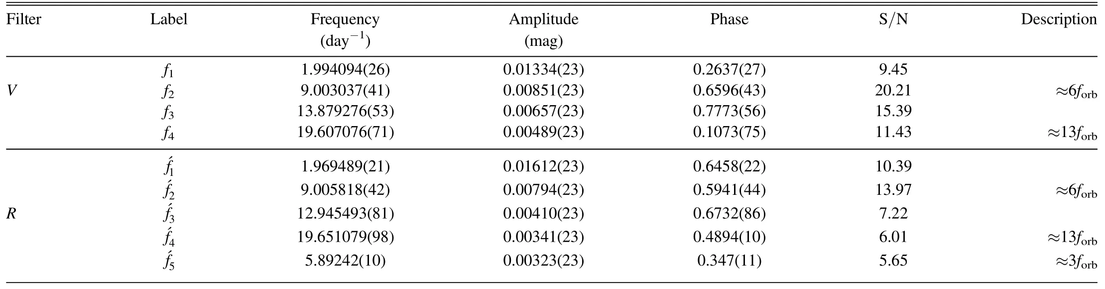
Period04 was used to find possible oscillation frequencies of the residuals.This program is commonly utilized to find frequencies in pulsating stars (Chen et al.2023; Kobzar et al.2023; Pothuneni et al.2023; Ulas & Ulusoy 2023).We calculate the frequency spectrum from 0 to 100 day−1.The Nyquist frequencies for V and R filters were obtained as 500 and 710, respectively.Because there was no significant frequency above 100 day−1in the frequency spectrum of these two filters, the frequency spectrum calculation window was considered from 0 to 100 day−1.Figures 10 and 11 display the frequency spectra obtained for V and R filters,respectively.We selected only frequencies that had a signal-to-noise ratio(S/N)greater than 4(Breger et al.1993).In Table 6,these frequencies are listed in order of occurrence.Four frequencies were found for the V filter and five for the R filter.

Figures 8 and 9 show the fitting of the detected frequencies to the residuals of the simulated light curve after subtracting from the observational data in V and R filters, respectively.In addition,the final residuals can be seen in these figures.For the V and R filters, the values ofwere obtained as 0.68 and 0.80, respectively.Therefore, the final residuals are better and their variances are reduced with respect to the initial data while the points are almost randomly distributed around the zero line.

6.Discussion and Conclusion

In this research, the light curves of the eclipsing binary system RS Sct were obtained in V and R Johnson-Cousins filters.Furthermore, the physical and orbital parameters of this system were determined by simultaneously analyzing the light and radial velocity curves.These results and the results of Buckley’s analysis are given in Table 2.There are two important differences between these results: (1) In the present research, for the first time, the photometric and radial velocity data were analyzed simultaneously using the mass ratio obtained from spectroscopic observations, while Buckley did not use this technique in the photometric data analysis.(2) As Buckley mentioned,due to the low quality of the data,he could not determine with certainty whether RS Sct is of detached or semi-detached type,so he assumed that the system is detached.However, in the present research, more accurate photometric data and simultaneous analysis of light and radial velocity curves were used to show that the system has a semi-detached configuration.This is also confirmed by the position of RS Sct in the diagram of orbital angular momentum versus total mass(Figure 6).The remarkable thing about the geometry of RS Sct is that the secondary component is on the verge of filling its inner Roche lobe and turning this system into a contact system.

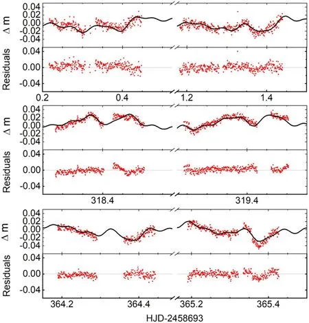
Figure 9.The residuals of the light curve between the model and observations(points)and the simulated curve with frequencies f1́, f2́, f3́, f4́and f5́(line)in filter R.Also, the final residuals are displayed at the bottom of the graphs.

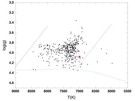
Table 3 presents the absolute parameters of this system,which are determined using the radial velocity data obtained by King & Hilditch (1984) along with the results of Dryomova et al.(2005).Dryomova et al.obtained the absolute parameters of this system by combining the results reported by King &Hilditch (1984) and Buckley (1984).However, due to the low accuracy of Buckley’s results, the absolute parameters related to the results reported by these authors also have spread.For the reasons mentioned before,perhaps the results of the present research are more reliable.By determining the absolute physical parameters of the components of this system, the locations of the primary and secondary components were found in the H-R diagram (Figure 4) and the color index–density diagram(Figure 5).In Figures 4 and 5,the primary component is close to the TAMS, indicating that the (more massive)primary component is at the beginning of its evolutionary stage and exits the main sequence.The O −C curve of the eclipse minima of this system was plotted.The parabolic form of the O −C curve can be attributed to the conserved mass transfer between the components.The rate of orbital period change and the rate of mass transfer from the primary to the secondary star were also determined.After removing the effect of mass transfer from the O −C curve, a periodic behavior was observed in the residuals.By fitting two light-time functions to the residuals, it was suggested that the periodic changes could have resulted from the presence of third and fourth components.After raising the possibility of additional components in this system, the light curves were reanalyzed.This time, the light of the third object was left free in the analysis of the light curves, but its effect on the light curves was estimated to be less than 1%,which can be ignored due to the dispersion of the data.Therefore, the possible third and fourth components should not have significant light.The minimum mass obtained for these components is in the mass range of dwarfs, 0.2M⊙

Figure 11.Fourier frequency spectrum obtained for the residuals by subtracting the simulated light curve from the observational data in the R filter.

Figure 12.Surface gravity vs.temperature.The position of the primary component of RS Sct is marked in purple.The green line represents the ZAMS,and the blue and red lines signify the hot and cold boundaries of the theoretical instability band for delta Scuti stars,respectively(Rodriguez&Breger 2001).Some pulsators of the delta Scuti type (black dots) are also shown in the diagram for comparison (Qian et al.2018).

The issue raised by Cook (1992) regarding the extreme changes of the RS Sct light and change in the primary eclipse depth by about a half magnitude was investigated.However,in the present research, the photometry of RS Sct was carried out for two years during which no signs of extreme light changes or change in the primary eclipse depth were observed.

The periodic behavior was investigated in the residuals after subtracting the simulated light curve from the observational data in the V and R filters.We detected four frequencies in the V filter and five in the R filter with an S/N greater than 4(Table 6).The frequencies f2and f4correspond to the V filter, and the frequenciesandcorrespond to the R filter.These frequencies are multiples of the orbital frequency(=1.505487041 day−1), so they may be caused by orbital motion and apsidal forces (Maceroni et al.2009; Fuller 2017)or by imperfect modeling of the binary light curve.The frequencies f1and f3in the V filter and́and́in the R filter are independent from each other.With a high probability,these frequencies may be due to the stellar pulsation in one or both components of the RS Sct binary system.Another possibility for the origin of most dominant frequencies f1and́can be the differential rotation of stars(with spots or surface inhomogeneities) or stellar activity (in the presence of a magnetic field).However, we cannot find any sign of spot or surface inhomogeneities in the light curve analysis, so the possibility of these issues is less.Also, gravity-mode (gmode) pulsations can be considered as an origin of f1and́.The frequencýis also not an independent frequency because it is a multiple of́.

The range of magnitude changes for these frequencies is between 0.003 and 0.017, which is in the range of delta Scuti stars.In addition, except for f1and́, it is found that other frequencies are in the usual frequency range of delta Scuti stars(5–100) (Grigahcene et al.2010).These pieces of evidence indicate that the pulsating component (or components) in this system is probably of the delta-Scuti type.

Moreover, the position of the primary component in the graph of surface gravity versus temperature (Figure 12) shows that this component is located within the instability band and in the range of delta Scuti pulsators.Therefore, the resultsobtained from the pulsation frequency analysis are confirmed.This indicates that probably the pulsating component in this system is the primary component and it is of delta Scuti type.

Table 6 Index Frequencies Obtained for V and R Filters After Removing Orbital Motion Effects

Acknowledgments

The authors would like to acknowledge the financial support of University of Birjand for this research under contract number 1399/D/ 6211.

Data Availability

The data underlying this paper will be shared on reasonable request to the corresponding author.