Stability and Convergence of Non-standard Finite Difference Method for Space Fractional Partial Differential Equation

WANG Qi(王琦),LIU Ziting(刘子婷)

(School of Mathematics and Statistics, Guangdong University of Technology,Guangzhou 510006, China)

Abstract: In this paper the numerical solution of the space fractional partial differential equation is derived by means of a non-standard finite difference method,and some corresponding numerical studies are investigated.For the two space fractional derivatives,we adopt the Gru¨nwald-Letnikov formula and the shift Gru¨nwald-Letnikov formula to discretize them,respectively.The non-standard finite difference scheme is constructed by denominator function with time and spacial steps.Furthermore,the stability and the convergence of this scheme are studied by the method of von Neumann analysis.Some new results are given.Numerical examples confirm that this scheme is effective for solving the space fractional partial differential equation.

Key words: Space fractional partial differential equation;Non-standard finite difference method;Stability;Convergence

1.Introduction

Fractional derivatives can effectively describe natural processes with memory and genetic characteristics because of their non-locality property.In recent decades,fractional partial differential equations have been widely used in many fields,such as control engineering,physical mechanics,biology and computer science[1-4].Space fractional partial differential equations(SFPDEs)are often used to model super-diffusion,where a particle plume spreads faster than predicted by the classical Brownian motion model.It is not easy to evaluate the fractional derivative for most functions.Because of the analytic solutions of most of SFPDEs cannot be obtained,so it becomes important to develop numerical methods for this type of equations.CHEN et al.[5]considered a SFPDEs with fractional diffusion and integer advection term,a fully discrete scheme was obtained by combining the Legendre spectral with Crank-Nicolson methods.They further proved that the scheme is unconditionally stable and convergent.ZHAO and WANG[6]developed a finite difference method (FDM) for space-time fractional partial differential equations in three dimensions with a combination of Dirichlet and fractional Neumann boundary conditions,by analyzing the structure of the stiffness matrix in numerical discretization as well as the coupling in the time direction,a fast FDM was obtained.Saw and Kumar[7]combined the Chebyshev collocation method with FDM to study one-dimensional SFPDEs,they attenuated the equations to a system of differential equations and solved them by iterative method.Bansu and Kumar[8]established a meshless approach for solving the space and time fractional telegraph equation,and the convergence of the scheme was discussed.Based on fourth-order matrix transfer technique for spatial discretization and fourth-order exponential time differencing Runge-Kutta for temporal discretization,Alzahrani et al.[9]developed two high-order methods for space-fractional reaction-diffusion equations.Owolabi[10]proposed an adaptable difference method for the approximation of the derivatives in fractional-order reaction-diffusion equations,the maximum error and relative error were both analyzed.Bolin et al.[11]studied a standard finite element method to discretize fractional elliptic stochastic partial differential equations,the strong mean-square error was analyzed and an explicit rate of convergence was derived.Iyiola et al.[12]provided a novel exponential time differencing method for nonlinear Riesz space fractional reaction-diffusion equation with homogeneous Dirichlet boundary condition,the numerical stability was examined.Takeuchi et al.[13]described a second-order accurate finite difference scheme for SFPDEs,it is proved that the difference scheme is second-order convergent,and the conditions for the stability of the scheme were given.Recently,a spectral method based on the use of the temporal discretization by the Jacobi polynomials and the spatial discretization by the Legendre polynomials was proposed by ZHANG et al.[14]for the numerical solution of time-space-fractional Fokker-Planck initial-boundary value problem.Later,semi-implicit spectral approximations for nonlinear Caputo time-and Riesz space-fractional diffusion equations were investigated in [15],the unconditional stability and the convergence of the fully discrete schemes were proved.Recently,Zhang and Lv[16]introduced a kind of regularization method to get rid of the ill-posedness for a space-fractional diffusion problem,the convergence and stability of the method were discussed.

In the late 1980s,Mickens[17-18]proposed a numerical method for solving differential equations: the non-standard finite difference (NSFD) method.The NSFD method has the potential to be dynamically consistent with the properties of the continuous model.Using this method,spurious solutions and numerical instabilities can be removed,and correct numerical solutions are qualitatively achieved for every time-step size.The NSFD method has already been used in the numerical simulation of fractional differential equations[19-23].Different from the above papers,we will study the stability and convergence of NSFD method for the SFPDEs with two fractional derivatives,the corresponding results are given.

In this paper,we consider the following SFPDEs

The main objective of this paper is to propose a NSFD method for solving the SFPDEs(1.1).This technique is based on the Gru¨nwald-Letnikov formula and the shift Gru¨nwald-Letnikov formula.Numerical simulations confirm that the proposed NSFD method is also successful in solving the SFPDEs.

The rest of the paper is organized as follows.In the next section we apply the NSFD method to solve the SFPDEs,where the NSFD method and the Crank-Nicolson FDM are combined together.Sections 3 and 4 give a detailed theoretical analysis of the stability and convergence of the scheme.Some numerical examples and comparisons are presented in Section 5 to demonstrate the accuracy and efficiency of the NSFD method.

2.Non-standard Finite Difference Scheme

In this section,we deduce the discrete scheme for (1.1) using the NSFD method.

Leth=L/mbe the space step,xj=jh,j=0,1,···,m,andτbe the time step,tn=nτ,n=0,1,2,···.Consider (1.1) at node (xj,tn)

whereRis local truncation error.

According to the NSFD method,we use more complicated “denominator function”ϕ1(τ)=τ+O(τ2) andϕ2(h)=h+O(h2) to replaceτandhin (2.2),so we get

Iis an unit matrix of (m-1)×(m-1) and the elements ofA(m-1)×(m-1)are as follows

3.Stability Analysis

In this section,we will analyze the stability of the NSFD scheme by von Neumann method.

Theorem 3.1The solution of (2.4) exists and is unique.

ProofAssuming thatλis the eigenvalue of matrixAandX0 is the corresponding eigenvector,that is,AX=λX.Define

Sinceλis the eigenvalue of matrixA,so (1-λ)/(1+λ) is the eigenvalue of matrix(I+A)-1(I-A) and|(1-λ)/(1+λ)|<1.Thus the spectral radius of (I+A)-1(I-A) is less than one,this completes the proof.

Theorem 3.2The scheme (2.4) is unconditionally von Neumann stable for 0<α<1 and 1<β<2.

whereiis an imaginary unit andqis a spatial wave number,substituting (3.3) into (3.2),we obtain

We first prove that the real part ofis positive,i.e.,

therefore (3.7) holds.The proof is finished.

4.Convergence Analysis

In this section,we will consider the convergence of the NSFD method.

Theorem4.1Assume thatu(xj,tn) is the solution of (1.1)at(xj,tn)andis the solutionof(2.4)at(xj,tn),respectively.Then the difference scheme(2.4)is unconditionally convergent.

ProofWe first compute the order of the local truncation error.In fact

5.Numerical Experiments

In this section,we give several numerical examples to illustrate the above theoretical results.

The analytic solution of (5.1) is given byu(x,t)=e-πtx3(1-x).

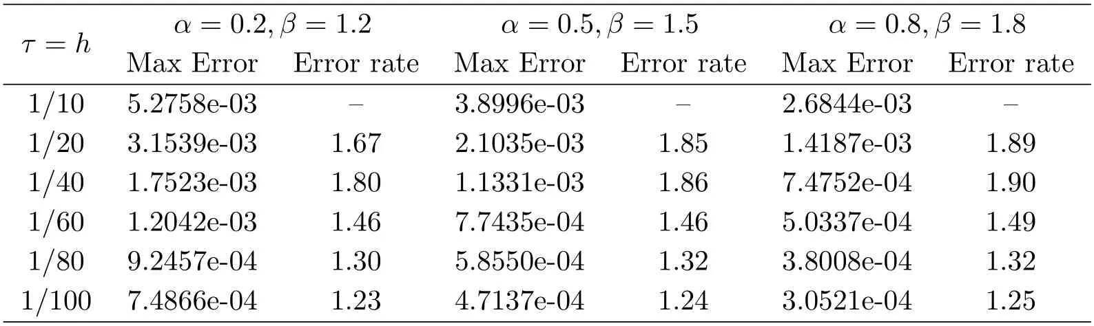
Firstly,letϕ1(τ)=τandϕ2(h)=h.Fig.5.1 shows the analytic solution and the numerical solution of (5.1) fort ∈[0,6].It is clear that,the numerical solution is in excellent agreement with the analytic solution.At the same time,both the analytic solution and the numerical solution are asymptotically stable.In Tab.5.1 we list the maximum error and error rate atT=1.From this table we can see that the NSFD method is convergent with orderO(τ2+h).Here we should note that the numerical method in the current situation is exactly the standard FDM,so the result is known to all.Furthermore,we find that the larger the values ofαandβ,the smaller the maximum error.

Tab.5.1 The maximum error and error rate for (5.1) with ϕ1(τ)=τ, ϕ2(h)=h, T=1

Fig.5.1 The analytic solution (left) and the numerical solution (right) of (5.1) with ϕ1(τ)=τ, ϕ2(h)=h and T=6

Secondly,setϕ1(τ)=1-e-τandϕ2(h)=h.The analytic solution and the numerical solution of (5.1) fort ∈[0,6] are shown in Fig.5.2.It can be seen from this figure that the numerical solution is asymptotically stable.Then the maximum error and error rate are given in Tab.5.2.From this table we know that the numerical method is also convergent with orderO(τ2+h).From comparing Tab.5.1 with Tab.5.2,it is easy to see that the maximum error is decreasing.

Tab.5.2 The maximum error and error rate for (5.1) with ϕ1(τ)=1-e-τ,ϕ2(h)=h, T=1

Fig.5.2 The analytic solution (left) and the numerical solution (right) of (5.1) with ϕ1(τ)=1-e-τ, ϕ2(h)=h and T=6

Thirdly,let the time denominator function remain unchanged and the spatial denominator function changes based on the second case.Specifically,letϕ1(τ)=1-e-τandϕ2(h)=eh-1.We plot the analytic solution and the numerical solution of (5.1) in Fig.5.3.Obviously,the numerical solution is asymptotically stable.Further,we list the maximum error and error rate in Tab.5.3 atT=1.From this table we know that the NSFD method is also convergent with orderO(τ2+h).Comparing the three tables,we can see that the maximum error continue to decrease,which shows that the maximum error can be reduced by changing denominator function.

Tab.5.3 The maximum error and error rate for (5.1) with ϕ1(τ)=1-e-τ,ϕ2(h)=eh-1, T=1

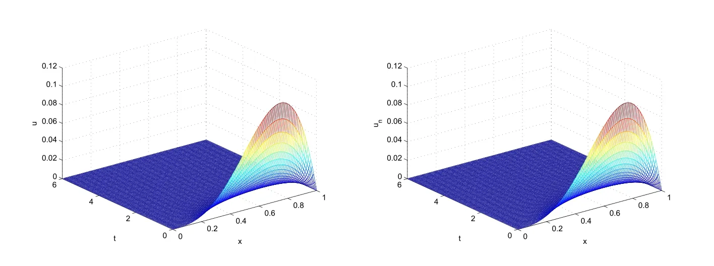
Fig.5.3 The analytic solution (left) and the numerical solution (right) of (5.1) with ϕ1(τ)=1-e-τ, ϕ2(h)=eh-1 and T=6

In summary,the choice of the denominator function is not unique,and the selection of appropriate denominator function can reduce the maximum error.From the above figures and tables,it can be seen that the NSFD method is convergent and preserves the stability of the original equation.