The Change Features of the West Boundary Bifurcation Line of the North Equatorial Current in the Pacific

GUO Junru, LIU Yulong, SONG Jun, 5), *, BAO Xianwen, LI Yan, CHEN Shaoyang, and YANG Jinkun



The Change Features of the West Boundary Bifurcation Line of the North Equatorial Current in the Pacific

GUO Junru1), 2), 4), LIU Yulong3), SONG Jun3), 5), *, BAO Xianwen1), 5), LI Yan3), CHEN Shaoyang3), and YANG Jinkun3)

1),,266100,2),100194,3),300171,4),,,, ACT2602,5),,266100,

The equatorial Current in the North Pacific (NEC) is an upper layer westward ocean current, which flows to the west boundary of the ocean, east of the Philippines, and bifurcates into the northerly Kuroshio and the main body of the southerly Mindanao current. Thus, NEC is both the south branch of the Subtropical Circulation and the north branch of the Tropical Circulation. The junction of the two branches extends to the west boundary to connect the bifurcation points forming the bifurcation line. The position of the North Pacific Equatorial Current bifurcation line of the surface determines the exchange between and the distribution of subtropical and tropical circulations, thus affecting the local or global climate. A new identification method to track the line and the bifurcation channel was used in this study, focusing on the climatological characteristics of the western boundary of the North Equatorial Current bifurcation line. The long-term average NEC west boundary bifurcation line shifts northwards with depth. In terms of seasonal variation, the average position of the western boundary of the bifurcation line is southernmost in June and northernmost in December, while in terms of interannual variation, from spring to winter in the years when ENSO is developing, the position of the west boundary bifurcation line of NEC is relatively to the north (south) in EI Niño (La Niña) years as compared to normal years.

North Equatorial Current; Pacific Ocean; bifurcation line; climate change; ENSO

1 Introduction

NEC system connects the subtropical and tropical cy- clones in the Pacific and makes important contributions to the heat budget in the western Pacific warm pool (Qu, 1997), while the warm pool is a key region that affects the circulation of ENSO (Webster and Lukas, 1992). The western boundary current systems of NEC directly enters the global thermohaline circulation through the Indone- sian throughflow (Gordon, 1986) and plays a decisive role in the meridional transport of heat, salt and mass in the world oceans (Qu, 1998). The western Pacific region is an intersection for the middle and high latitude water masses (Fine, 1994), from which the concept of subtropical cell is derived: The net heating from the low latitude ocean is transported northwards from the surface to the NEC and then via Kuroshio to the higher latitudes; while the cold subsurface/deep water water flows southwards in the thermocline and then to the trop- ics through different passageways after being bifurcated by the NEC (Lu, 1998; Johnson and Mcphaden, 1999); and lastly turns upwards at the equator, constitute- ing the sallow meridional overturning circulation (Mc- Creary and Lu, 1994; Liu, 1994). The NEC links the sub- tropical and tropical regions, and is the boundary between subtropical and tropical circulations. At the western bound- ary, NEC bifurcates into two branches: NEC north branch passageway (flowing to Kuroshio) and NEC south branch passageway (flowing to the Mindanao current) (Xu and M-Rizzoli, 2013). There are different bifurcation points of NEC at different depths, the line connecting these bi- furcation points is the bifurcation line which determines the distribution of mass, heat and salt between the sub- tropical and tropical circulations. The interannual and decadal changes of the NEC bifurcation line can affect the tropical and subtropical heat distribution and thermal structure change, thus affecting the local or global climate (Song, 2011). Therefore, the change of the NEC bifurcation line plays a very important role in our re- search on the global climate change. Previous studies mostly focus on the change of the western boundary bifurcation points and less research is made on the change pattern of the bifurcation points, but this charac- teristic of bifurcation line can more directly and accu- rately identify the change of circulation systems (Wang and Liu, 2000).

The position of the bifurcation point of NEC plays an important role in the Climate Change, so the research on the latitude of the NEC bifurcation point began as early as in the 1970s. According to the hydrological observations in 1934–1968, Nitani (1972) held that the surface of the NEC bifurcation point is about between 11˚N and 14.5˚N and the position of the bifurcation point moves north- wards with the increase of depth. Through analysis of the distribution of water masses, Toole(1988) estimated that the latitude of bifurcation was about 12˚N. From the hydrological data from the Sino-American Joint Survey between September, 1987 and April, 1988, Toole(1990) defined the latitude where the transport flow func- tion is zero and concluded that the bifurcation latitude was near 13˚N. Employing the model results, Qiu and Lukas (1996) defined the latitude where the average me- ridional speed is zero within the zone of two degrees of latitude along the western boundary and concluded that the bifurcation latitude was close to 13˚N. According to the results of model calculation, Metzger and Hurlburt (1996) concluded that the average position of NEC moved in 15.6˚N±0.6˚N, shifting northwards with depth and reaching 18˚N at the depth of 700m. On the basis of the climatic data of temperature and salinity, Qu(1999) defined the place where the average meridional speed is zero within two degrees of longitude from the coast as the position of bifurcation and concluded that near the surface the bifurcation line was at 13.5˚N, at 500m in 18˚N and the vertical average position between 0–500m was in about 15˚N. By using the WOA (1994) historical observations, Qu(1999) concluded that in the upper thermocline, the NEC bifurcation point was at 15˚N, moved northwards with depth and on the 27.2kgm−3isopycnic surface (about 800m), reached 20˚N. By analysing the historical observations (WOA98), Qu and Lukas (2002) defined the latitude where the merid- ional transport within 5 degrees of longitude from the western boundary is zero as the latitude of bifurcation point and concluded that near the surface within 100m it was at 14˚N, shifted northwards with depth and reached 23˚N at 800m. By using the data of world ocean tempera- ture, salinity and dissolved oxygen in 1998 of WOD, Qu and Lukas (2003) found that the average position of the bifurcation latitude near surface (within 100 m) is 14.2˚N, and if the effect of Ekman transport is added, it moves to 13.3˚N while the bifurcation latitude shifts northwards with depth and at the depth of 800m, it is located in 20˚N. Based on the calculated results of the model, Yaremchuk and Qu (2004) defined the latitude of the mean merid- ional speed change symbol and it was derived from cal- culation that the NEC average position is 14.3˚±0.7˚N. By employing the computed results of the high resolution OGCM model, Kim(2004) defined the latitude where the average meridional speed is zero within two degrees of longitude away from the coast of the Philip- pines as the bifurcation latitude and obtained the annual average bifurcation latitude of 15.5˚N, which shifts northwards with depth, and the bifurcation latitude moves from 14.3˚N at the surface to 16.6˚N at 500 m. By use of the WOCE drifting buoy data in 1987–1998, Li(2005) defined that the position of the bifurcation point is between the trajectories of the buoy west of 130˚E turning southwards and northwards. And in the case of the trajec- tories of the buoy turning southwards and northwards that cross west of 130˚E, the latitude of the bifurcation point is defined as the latitude where the buoy trajectories cross and the surface bifurcation latitude is estimated to be between 11˚N and 14.7˚N. Wang and Hu (2006) used the satellite altimeter data (October, 1992–December, 2004) and concluded that the bifurcation latitude at the NEC western boundary surface is located at 13.4˚N. Zhang(2008) used the satellite altimeter data of high spatial and temporal resolution to calculate the geostrophic current and defined the average latitude where the velocity gradient quickly increases and the me- ridional velocity is zero when reaching the shore as the criterion by which to determine the latitude of bifurcation. And the annual average bifurcation latitude was estimated to be 13.4˚N.

It can be seen that scientists (Zhai and Hu, 2012) have done a lot of researches on the flow field structure and bifurcation position of the western boundary current system, but most scholars located the bifurcation point in terms of the meridional velocity of the flow field, and as there are many factors affecting NEC and the change is complex, the difference in the results obtained from choosing to average over different width ranges is greater (Kim, 2004). Furthermore, even if the position of bifurcation point is determined, it is still impossible to reflect very well the bifurcation situation of the whole current system and obtain more detailed bifurcation fea- tures of the flow field. Hang and Wang (2001) and Wang and Huang (2005) proposed the method of quantitatively describing the barotrophic sea channel by wind stress, and that of quantitatively describing the baroclinic channel in recent years, by which to research into and analyse the property of the channel transport change with latitude. However, they did not make further research on the fea- tures of the bifurcation line.

This paper compared the north Equatorial Current in the Pacific and tried to overcome the above mentioned shortcoming by using a new computational method,, identifying the position and change of bifurcation at each layer by calculating the isopycnal line, describing the NEC bifurcation line and making systematic analysis of its form and change pattern, analysing the plane distribu- tion of the bifurcation line on the two-dimensional plane, stratifying the data to obtain the vertical distribution of bifurcation lines and lastly deriving the climatic, seasonal and interannual changes of the bifurcation line though statistical analysis.

2 Data and Methods

2.1 Data Description

This paper used the SODA (Simple Ocean Data As- similation) database version 2.0.2 (Carton and Giese, 2005), which is based on the GFDL (Geophysical Fluid Dynamics Laboratory) reanalysis data of the Parallel Ocean Program physics marine numerical model and data assimilation technology.

This model includes the terrigenous freshwater flux with vertical resolution of 10m near the surface. The model’s wind stress forcing field is constructed by the COADS (Comprehensive Ocean-Atmosphere Data Set) and NECP (National Centers for Environmental Predic- tion) data (after 1992), of which the long-term trend of wind stress data not in harmony with the sea surface pressure trend observed has been eliminated. For the spe- cific description of these datasets involved in the research, refer to Carton and Giese (2008). The SODA data prod- ucts covers the 50 years from 1958 to 2007, with the global longitude range from 0.25˚ to 360.25˚ (from west to east) and the latitudinal range from −75.25˚ to 89.25˚ (from south to north); the data have horizontal resolution 0.5˚×0.5˚ and are vertically divided into 40 layers. The horizontal and vertical resolutions are high enough for studying the bifurcation of NEC.

2.2 Method of Calculation and Data Processing

The sea area selected in this study is in the North Pa- cific (100.25˚E–120.25˚W, 2.25˚S–57.25˚N). The paper used the data on the equipotential density surface layer by layer for analyzing the path. The specific method of cal- culation is as follows:

The first step is to calculate the grid thermohaline data to get the potential temperature and density on thecoor- dinate (Except otherwise specified, the density or poten- tial density mentioned here after also represents the po- tential density). The layer-by-layer potential density av- eraged over the region is found and then the potential density layer is divided in equal intervals. In choosing the potential density layer, if it is too small, the low density water can only be reserved in the equatorial part of the west Pacific, which cannot display the path of water par- ticles; if it is too large, the bifurcation of western bound- ary trends to be blurred and disappears and so cannot be distinguished.

The second step is to carry out the coordinate trans- formation, turning thecoordinate of raw data into the isopycnal surface coordinate for our analysis. First, the multiple density stratification is used to carry out the multi-layer division in the density stratification range and the algorithm of interpolation is employed to calculate this density range, and the meridional velocity, zonal ve- locity, temperature and salinity in isopycnal layer. Then, the isopycnal layer thickness is chosen according to the weight to represent the range. For the expanded and den- sified density layer, filter value taking is carried out ac- cording to the weight (the difference in the distance to the calculation point), and again the calculation is done to the required isopycnal surface, thus obtaining the variable required for the calculation under the density coordinate.

The third step is to carry out the evaluation of integrals for the path with the nonlinear, high-order, one-step nu- merical algorithm of Runge-Kutta. The Runge-Kutta method is well-known as a multilevel algorithm, which is different from the integration method of ordinary differ- ential equations such as Adams-Bashorth, Adams-Monl- ton,(multiple methods) and it does not need to recal- culate the unknown function value of each order in the differential equation. It requires us to calculate the values offor a simple correction. The basic idea is to use the value of the intermediate step to replace the higher de- rivative.

This paper uses for the first time the isopycnal surface stream line tracing and judging algorithm (Lagrangian particle tracking technique is used in this study), giving the accurate trace points of the NEC northern branch channel and southern branch channel and its bifurcation line on the calculated level by starting from the grid ve- locity field and tracking the stream lines within the chan- nels at different density layers. If the same calculation is done for the density layers, we can get the whole three-dimensional NEC western boundary current system. So this paper gives for the first time the precisely quanti- fied structure of the NEC western boundary channel and its bifurcation condition.

3 Climatic Characteristics of the Pacific NEC Western Boundary Bifurcation Line

This paper does not adopt the more limited method of bifurcation point, rather the integration path method to obtain the bifurcation line in the research. Fig.1 gives the long-term averaged stratified bifurcation line of the NEC western boundary. In the layer-by-layer change, with the increase of depth, the bifurcation line shifts northwards, which is consistent with the previous findings that in the sense of annual average the latitude of the western boundary bifurcation point moves northwards from the surface to deep layers. For the bifurcation line used in this paper, its distribution form of being high in the west and low in the east may be seen and the layer-by-layer bifur- cation lines tend to be parallel, do not overlap in the ver- tical direction and density changes little in the deeper layers, so the degree of separation between bifurcation lines increases on the deep-layer isopycnal surface. The latitudinal difference of a simple bifurcation line between the east and west ends of 130˚E–170˚E is about 1.5˚.

For the poleward shift of the NEC western boundary bifurcation line with depth, we approach this phenomenon from the oceanic circulation basis. In the vorticity equa- tion, the motion reaches a constant state and at the same time the exogenous process can be neglected (large-scale motion):

Fig.1 Long-term averaged NEC western boundary stratification (23.4–26.4kgm−3) bifurcation lines.

whereωis absolute vorticity;is horizontal flow veloc- ity;is density,is pressure.

The relative vorticity of the large-scale motion is far smaller than the planetary vorticity:

whereis the Coriolis parameter.

The component form of baroclinic fluid may be ex- pressed as:

hereis zonal coordinate with east positive;is merid- ional coordinate with north positive;is vertical coordi- nate with down positive.

This is the thermogenic wind relationship, which con- structs the relationship between the variation of vertical flow velocity and the horizontal density (temperature), which is a very important relationship between flow ve- locity and density (temperature) in the ocean. Further- more, it is derived from the magnitude relation:

In the meantime, for the vertical flow velocity shear and horizontal density gradients, we have:

. (3-5)

As the gradient of salinity is smaller, when the density (temperature) increases polewards, the increase of the current with depth quickly produces the flow westwards, as a result of which, the centre of the subtropical gyre (anticyclonic) moves polewards with the increase of depth (Liu, 2011). Therefore, we get the image of the shift polewards of the western boundary bifurcation line with depth due to the effect of the subtropical gyre.

Figs.2 and 3 give the long-term averaged distribution of the NEC western boundary bifurcation lines in the sec- tion of 130˚E under thecoordinate and potential density coordinate. Under the depth coordinate it may be seen that the depth of the first layer density 23.4kgm−3 in the whole section of 130˚E over a span of 8˚N–25˚N between south and north is between 75m and 125m; on the depth coordinate are contained the information on the equal potential density line, isotherm and zonal velocity field. On the section of 130˚E near the western boundary, the isotherm and the isopycnal line are basically parallel. At the same time, the upper temperature gradient in the low latitude area is greater than that in the high latitude area and the isopycnal line is far shallower. For instance, the isopycnal line of 26.4kgm−3is 210m at about 8˚N, while at about 25˚N it amounts to 555m. It can be seen from the figure that the western boundary bifurcation latitude in this section is not at the extremum centre of zonal veloc- ity, but is to the north a little. On the section of depth co- ordinate, the depth from the first layer to the last layer totals 500m in depth; the bifurcation line latitude varies for about 4˚, with each 100m deepening the bifurcation latitude moves northwards for about 1 degree and the northward distance in the upper layer is slightly larger than that in the lower layer. In the density coordinates of Fig.3, the bifurcation line points shift in the density layer. As the upper layer is relatively thinner, the variation of bifurcation line points in the density coordinates is not obvious, while in the lower layer there is a distinct northward shift. This has been verified in Fig.2 in which in area of bifurcation line points, it may be clear that it is located at the largest bended location,, near the low-lying (deeper) place of the isopycnal surface.

Fig.2 Long-term averaged 130˚E sectional (depth coordinated) drawing, in which there are the NEC western boundary bifurcation lines (grey squares), isopycnal lines (solid lines) and equal zonal velocity lines (dotted lines).

Fig.3 Long-term averaged 130˚E sectional (depth coordinates) drawing, in which there are the NEC western boundary bifurcation lines (grey squares), isobaths lines (solid lines) and equal zonal transport lines (dotted lines).

4 Seasonal Variation Features of the NEC Western Boundary Bifurcation Line

Fig.4 gives the seasonal variations of the fine verti- cally-averaged NEC western boundary bifurcation line (23.4kgm−3–26.4kgm−3), derived on the basis of the channel algorithm. In winter (November, December and January), the bifurcation line is relatively straight and the difference in the latitude of bifurcation is not obvious in the east and west directions, which is related to the dis- tribution of NEC flow pattern in the winter, being about 15.7˚N on the average. The bifurcation line is located at the higher latitudes throughout the year, being northern- most in November. Starting from February it obviously begins to move southwards gradually, showing inclining state of being high in the east and lower in the west. In June the westernmost end of the bifurcation line moves to the southernmost position in the year, in about 14.3˚N on the average. This coincides with the findings of Qu and Lukas (2002) by use of the data on the west Pacific tem- perature, salinity, DO concentration,The research makes an integral calculation of the dynamic height and its corresponding circulation from surface to 1000 m, and in the light of the Ekman transport, concludes that the NEC bifurcation point begins to move southwards in January, reaches the southernmost end and then moves northwards, reaching the northernmost end in December. The time difference is mainly due to the different integra- tion methods used. This paper carries out the vertical in- tegration according to the density coordinate. And the calculated density layers are mostly within 100–600m, not including all the intervals of integration in 0–1000m. After June, the bifurcation line begins to shift northwards, the east-to-west dip is more obvious and the difference in latitude between the east and west ends of the line in au- tumn reaches the highest throughout the year, up to 2.8˚, while such difference in winter when the bifurcation line is relatively straight is only 0.9˚, and with the lapse of time, the bifurcation line moves northwards and the dip angle decreases gradually.

Fig.4 Seasonal variations of the vertically averaged NEC western boundary bifurcation line (23.4–26.4kgm−3).

Fig.5 is the seasonal variations of the NEC western boundary bifurcation lines layer by layer. In each sheet, there are 16 curves, representing the bifurcation lines in the 16 density layers. The distribution of the bifurcation lines on all the isopycnal surfaces in the whole area is relatively regular, and seasonally the latitude of bifurcation line moves northwards with depth and basically is parallel with the bifurcation line of the upper density layer. In winter, the bifurcation line is relatively higher in latitude and straight in shape while in summer and autumn it in- clines and at the west end of the line the wind direction changes and the wind stress magnitude is lower as com- pared with that in spring and winter. The location repre- sented by the first layer bifurcation line is not different from that indicated by the vertically averaged seasonal change,, it is moving northwards in winter and southwards in summer, being straight in winter and in- clining in autumn. The change in shape is displayed more obviously in the layer-by-layer bifurcation line. Among others, there exists a bifurcation line ridge layer by layer (the line bulges northwards), and the deviation of the ridge from the main axis of the bifurcation line may reach about 1.2˚; it belongs to an obvious abnormal fluctuation. Such phenomenon begins to appear and develops in March and April; it speeds up in July, the intensity being lower at about 168˚E, and in August propagates west- wards to 166˚E, with a tendency to increase. In Septem- ber, the ridge moves to 163˚E, further strengthening. By October, the ridge with the largest intensity has reached the location of 158˚E; in November the follow-up fluc- tuation of October forms another ridge, which propagates westwards; and the former ridge moves westwards to about 155˚E to form a double ridge with its intensity also dropping significantly. In December, the ridge propagates to the western boundary, which results in the up dip of the western boundary bifurcation point; and then it basically weakens and disappears. Figs.3–9 show the seasonal change in the NEC western boundary bifurcation line’s vertical dipping. A simple point-to-point method of inter- polation is used to treat the degree of diffusion of the layer-to-layer bifurcation line from bottom to surface along the longitudinal direction. The phenomenon with the maximum diffusion magnitude of the ridge in the whole calculated layer exceeding 4.4˚ appears in the spring and summer months of May and June, while the minimum magnitude of diffusion smaller than 2.1˚ occurs in the autumn months of September and October. It can be seen from the time evolution figure that the diffusion amplitude of the bifurcation line as a whole in January and February is smaller, the degree of diffusion is smaller, and the degree of diffusion in the western part of the line is even weaker than that in the eastern part. In March, the degree of diffusion of the bifurcation line in the vertical direction begins to increase and the amplitude fluctuation grows. By June, the vertical amplitude reaches the maxi- mum, generally exceeding 3.6˚ from west to east, which is the largest throughout the year. In July, the diffusion amplitude begins to drop and upon entering the autumn months of August, September and October, it contracts to the minimum level and part of the variation amplitude is as low as below 2.4˚, which is the smallest throughout the year. Starting from November, the vertical variation am- plitude of the NEC western boundary bifurcation line again grows gradually, so we can say that the diffusion amplitude of the bifurcation line varies regularly with season.

Fig.5 Seasonal variations of the layer-by-layer NEC western boundary bifurcation lines.

Fig.7 gives the latitudes of the Pacific NEC western boundary bifurcation line and the depth values corre- sponding to it. In terms of the movement of the western boundary bifurcation line, as far as the 140m and 160m depth lines are concerned, the 160m depth line is located near the surface in June, which shows the depth of the bifurcation line is the largest in June. And in December, the 140m depth line is located far away from the surface, showing that the bifurcation line in December is the shal- lowest. Fluctuations are constantly seen on the bifurcation line to propagate from west to east. Starting from May there are two obvious wave crests located at the longi- tudes of 145˚E and 170˚E from top to bottom, constantly propagating westwards. By October the wave crest propa- gating from 170˚E has developed most strongly while the 145˚E wave crest has propagated up to the western boundary, thus causing the bifurcation line within 10 de- grees of longitude of the western boundary to swing from the southwest-northeast direction in May to the north- west-southeast direction in December and lowest latitu- dinal position to shift from the western boundary to about 140˚E with a longitudinal difference of over 10 degrees.

From the layer-by-layer angle with time as the variation axis, it may be clearly seen that the latitudinal change propagates from west to east and that the depth is the largest at the lowest latitude. Another phenomenon is that the lowest latitude of the western boundary bifurcation occurs around June while the latitude at 145˚E which is the inflection point of the high value latitude propagation occurs around October, but at the bottom,, 26kgm−3, the lowest signal of the western boundary latitude occurs around July, the highest latitude is postponed to occur around November and possibly the signal that first changes propagates from the upper layer to the lower layer.

5 Response of the Location of the NEC Western Boundary Bifurcation Line to the ENSO Event

El Niño and La Niña years are chosen according to the Niño 3.4 exponent. The Niño 3.4 abnormal temperature maximum occurs in winter. The spring in the year when ENSO develops is usually chosen as the initial developing season and a multi-seasonal bifurcation line comparison is made with season as unit. Analysis is made according to four seasons of spring (March–May), summer (June–August), autumn (September–November) and winter (De- cember–February), which may be further divided into several time periods of the initial spring (March–May), developing summer (June–August), developing summer (June–August), developing autumn (September–Novem- ber), peak winter (December–February) and weakening spring (March–May) on the basis of the process of de- velopment-peak-weakening of ENSO and the variations of the bifurcation line are obtained from calculation as follows:

Figs.8–15 give separately the NEC western boundary bifurcation lines in the spring (initial), summer (develop- ing), autumn (developing), and winter (peak) in the year when ENSO occurs and those in the next year’s spring (weakening), summer (weakening), autumn (weakening), and in the figures, the three lines indicate the El Niño year (Red Line), La Niña year (Blue Line), Long-Term Average (Black Line). It is usually believed that the spring of the year when ENSO occurs is the period when ENSO begins to develop, and in the spring of developing period, the upper bifurcation line first appears in the east to north in the form that it is higher (lower) of latitude in the El Niño (La Niña) year relative to normal years. With the change of seasons, up to the summer of the year when ENSO occurs, the three bifurcation line are completely separated from each other, the highest (lowest) latitude in the El Niño (La Niña) year. The bottom flow pattern is confused in the La Niña year and the situation in autumn is similar to that in summer, which will not be discussed in detail. The winter bifurcation lines in the year when ENSO occurs come back to the average state, the separa- tion degree at the east ends of the three bifurcation lines is reduced, the bifurcation lines begin to draw near, but their west ends still have a higher degree of separation, which is in consistent with the developing period.

Fig.7 NEC western boundary bifurcating line and the variations at its corresponding depths (the shadow part is the latitude values at the two ends of the line).

Fig.8 NEC western boundary bifurcation line in the initial spring: El Niño year (red line), La Niña year (blue line), long-term average (black line).

In the spring of the second year when ENSO occurs, the signed of the bifurcation line in the east by south (by north) further increases, propagating westwards to around 150˚N, higher (lower) in the west in the El Niño year (La Niña year),which the bifurcation line in average years is located in the middle. The main intersection point of the summer bifurcation lines in the second year propagates up to the western boundary. In other parts except the western boundary, the El Niño (La Niña) year’s lower (higher) average lines are in the middle, and in the El Niño year there appear obvious fluctuation ridges of bi- furcation lines, the distribution patterns being basically constant in the upper and lower layers. In the second year’s autumn following the year when ENSO occurs, the bifurcation line transforms into the state where the El Niño (La Niña) year’s lower (higher) average line is in the middle, and in the meanwhile, the fluctuating peak formed in summer continues to propagate west wards, and the fluctuation in the El Niño year is stronger than that in the La Niña year. In the second year’s winter fol- lowing the year when ENSO occurs, the relative average value of the ENSO occurs, the relative average value of the NEC western boundary bifurcation line falls as a whole and in the following season returns to normal. By then, this ENSO event has ended.

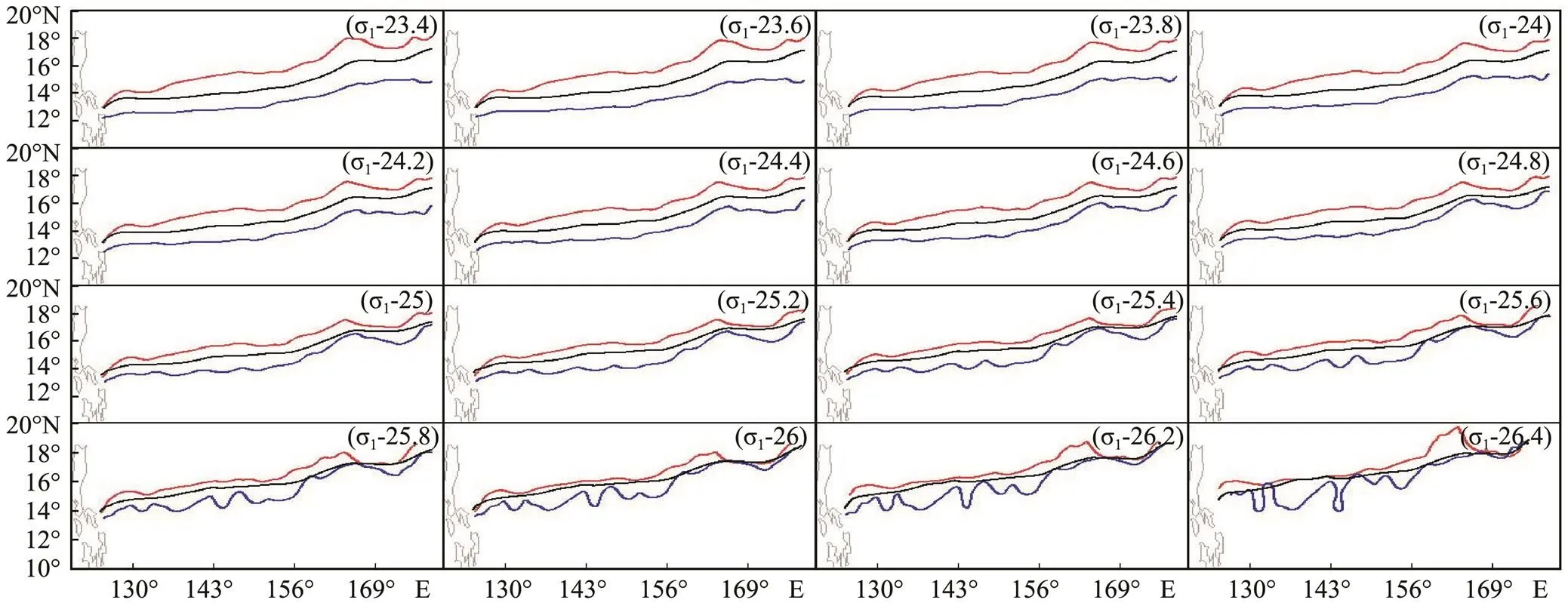
Fig.9 NEC western boundary bifurcation line in the developing summer: El Niño year (red line), La Niña year (blue line), long-term average (black line).

Fig.10 NEC western boundary bifurcation line in the developing autumn: El Niño year (red line), La Niña year (blue line), long-term average (black line).

Fig.11 NEC western boundary bifurcation line in the peak winter: El Niño year (red line), La Niña year (blue line), long-term average (black line).

Fig.12 NEC western boundary bifurcation line in the weakening spring: El Niño year (red line), La Niña year (blue line), long-term average (black line).

Fig.13 NEC western boundary bifurcation line in the weakening summer: El Niño year (red line), La Niña year (blue line), long-term average (black line).

Fig.14 NEC western boundary bifurcation line in the weakening autumn: El Niño year (red line), La Niña year (blue line), long-term average (black line).

Fig.15 NEC western boundary bifurcation line in the weakening winter: El Niño year (red line), La Niña year (blue line), long-term average (black line).

6 Conclusions

By use of the SODA data, this paper studies the cli- matic, interannual and seasonal variations of the NEC western boundary bifurcation line. It gives a visual dis- play of the channel bifurcation line proposed by this paper, makes an analysis of the position and its physical quantity change and obtains the following results with regularity:

1) The long-term averaged NEC western boundary bi- furcation line shifts northwards with depth, and its main mechanism could be explained by the thermal wind rela- tionship in the ocean. The western boundary point of the bifurcation line is from 13.8˚N of the 23.4kgm−3isopy- cnal surface to 17.7˚N of the 26.4kgm−3isopycnal sur- face. It may be seen from the sections in different longi- tudes: with each 100 meters deepening, the latitudinal bifurcation moves northwards for about 1 degree and the northward shifting distance in the upper layer is slightly larger than that in the lower layer. The bifurcation line is located north of the centre with the maximum meridional velocity and near the low-lying (deeper) place of the isopycnal surface.

2) The seasonal variation of the vertically averaged NEC western boundary bifurcation line is characterized by south-north moving and east-west dipping on the whole and the western boundary bifurcation point is a part of the whole movement of the bifurcation line. In terms of the zonal position of bifurcation line, it is north- ernmost in December with an average latitude of 15.7˚N; In June, it is southernmost with an average latitude of about 14.3˚N. The difference in the winter bifurcation latitude in the east and west directions is not obvious and the bifurcation line is relatively straight; The spring bi- furcation line begins to show a dipping state of being high in the east and low in the west, and the autumn latitudinal difference in the east and west directions is as large as over 2.8˚.

3) The seasonal variation of the NEC western boundary bifurcation line has a significant feature of the fluctuation propagating westwards, indicating that the bifurcation point is obviously modulated by the westward propagate- ing fluctuation (Rossby wave). Starting from July, the ridge occurring at 168˚E (The bifurcation line bulges northwards) propagates westwards and is strengthened; it moves westwards in October to the place west of 158˚E, with the amplitude reaching the maximum; In November it continues to propagate westwards but its intensity is obviously weakened; in December it propagates to the western boundary where it is basically weakened and disappears. The bifurcation lines of deeper layers in No- vember and December have a shape of three ridges and two troughs, but at the surface this distribution of forms is not distinct. In terms of the south-north movement of the NEC western boundary bifurcation line, the signal of latitude change in the lower layer lags behind that in the upper layer and the westward propagation of the bifurca- tion line ridge may cause the western boundary bifurca- tion point to swing between south and north. The bifurca- tion line in each layer has a northward jump by a large margin (The average latitude of bifurcation line in each layer has a northward jump of over 1.6˚), which in time is in agreement with the first northward jump of the atmos- pheric subtropic high pressure system. In March the bi- furcation lines in all layers all withdraw to the south. Therefore the bifurcation lines may be divided into two clusters: being concentrated in the south in March–June and in the north in July–February. Corresponding to this, the average layer thickness of layers along the bifurcation line is also relatively small in March–June and larger in other months, which should be the result of vorticity conservation.

4) The interannual variation of the NEC western boundary bifurcation line shows that in the developing and strengthening period of El Niño (La Niña), the bifur- cation line is to the north (to the south). Base on the proc- ess of development-peak-weakening of ENSO, several time periods are divided,, initial spring (March–May), developing summer (June–August), developing summer (June–August), developing autumn (September–Novem- ber), peak winter (December–February) and weakening spring (March–May). In the initial spring of El Niño, the bifurcation line is first in the east by north; in the devel- oping summer and autumn, the whole bifurcation line is to the north and reaches the maximum. In the peak winter, the bifurcation line restores the average state and the east part begins to go by south; in the weakening spring, the signal in the east by south further increases and propa- gates westwards. During the La Niña, the development of the bifurcation line is similar, but in opposite phase. Dur- ing the ENSO, there is an obvious feature of propagating westwards. The phenomenon that the maximum south-north shift of the western boundary bifurcation line oc- curs before the prime period of ENSO deserves further study in the future.

Acknowledgements

This work was supported by the National Natural Sci- ence Foundation of China (41206013, 41106004, 41376014, 41430963); Key Marine Science Foundation of the State Oceanic Administration of China for Young Scholar (2013203, 2012202, 2012223); POL Visiting Fellowship Program (Jun Song); the Public Science and Technology ResearchFundsProjectsofOcean(201205018,201005019); China Scholarship Council ([2008]3019, [2012]3013).

Carton, J. A., and Giese, B. S., 2005. SODA: A reanalysis of ocean climate., 1: 1-30.

Carton, J. A., and Giese, B. S., 2008. A reanalysis of ocean climate using simple ocean data assimilation (SODA)., 136: 2999-3017.

Fine, R., Lukas, R., Bingham, F. M., Warner, M. J., and Gammon, R. H., 1994. The western equatorial Pacific is a water mass crossroads., 99: 25063-25080.

Gordon, A. L., 1986. Interocean exchange of thermocline water., 91: 5037-5046.

Huang, R. X., and Wang, Q., 2001. Interior communication from the subtropical to the tropical oceans., 31: 3538-3550.

Johnson, G. C., and McPhaden, M. J., 1999. Interiod pycnocline flow from the subtropical to the equatorial Pacific Ocean., 29: 3073-3089.

Kim, Y. Y., Qu, T., and Jensen, T, 2004. Seasonal and interannual variations of the North Equatorial Current bifurcation in a high-resolution OGCM., 109, C03040.

Li, L. J., Liu, Q. Y., and Liu, W., 2005. Surface current speed andbifurcation of the North Equatorial Current in the Pacific Ocean., 35 (3): 370-374.

Liu, Y. L., Wang, Q., Song, J., Zhu, X. D., Gong, X. Q., and Wu, F., 2011. Numerical study on the bifurcation of the North Equatorial Current., 10 (4): 305-313.

Liu, Z., 1994. A simple model of the mass exchange between the subtropical and tropical ocean., 24: 1153-1165.

Lu, P., McCreary, J. P., and Klinger, B. A., 1998. Meridional circulation cell and the source water of the Pacific equatorial undercurrent., 28:62-84.

McCreary, J. P., and Lu, P., 1994. On the interaction between the subtropical and equatorial ocean circulation: The subtropical cell., 24: 466-497.

Metzger, E. J., and Hurlburt, H. E., 1996. Coupled dynamics of the South China Sea, the Sulu Sea, and the Pacific Ocean., 101: 12331-12352.

Nitani, H., 1972.. University of Washington Press, Washington, 129-163.

Qiu, B., and Lukas, R., 1996. Seasonal and interannual variability of the North Equatorial Current, the Mindanao Current, and the Kuroshio along the Pacific western boundary., 101: 12315-12330.

Qu, T. D., Meyers, J. G., and Godfrey, S., 1997. Upper ocean dynamics and its role in maintaining the annual mean western Pacific warm pool in a global GCM., 17: 711-724.

Qu, T. D., Mitsudera, H., and Yamagata, T., 1998. On the western boundary currents in the Philippine Sea., 103 (4): 7537-7548.

Qu, T. D., Mitsudera, H., and Yamagata, T., 1999. A climatology of the circulation and water mass distribution near the Phi- lippine coast., 29: 1488-1505.

Qu, T., and Lukas, R., 2002. Depth distribution of the subtropical Gyre in the North Pacific., 58 (3): 525-529.

Qu, T., and Lukas, R., 2003. The bifurcation of the North Equatorial Current in the Pacific., 33: 5-18.

Song, J., Xue, H. J., Bao, X. W., and Wu, D. X., 2011. A spectral mixture model analysis of the Kuroshio variability and the water exchange between the Kuroshio and the East China Sea., 29 (2): 446-459.

Toole, J. M., Zou, E., and Millard, R. C., 1988. On the circulation of the upper waters in the western equatorial Pacific Ocean., 35: 1451-1482.

Toole, J., Millard, C., Wang, Z., and Pu, S., 1990. Observations of the Pacific North Equatorial Current bifurcation at the Philippine coast., 20: 307-318.

Wang, Q., and Huang, R. X., 2005. Decadal variability of pycnocline flows from the subtropical to the equatorial Pacific., 35 (10): 1861-1875.

Wang, Q., and Liu, Q. Y., 2000. The study on the Pacific Subtropical Cell., 1: 1-5.

Wang, Q. Y., and Hu, D. X., 2006. Bifurcation of the North Equatorial Current derived from altimetry in the Pacific Ocean., 18 (5): 620-626.

Webster, P. J., and Lukas, R., 1992. TOGA/COARE: The coupledocean-atmosphere response experiment., 73: 1377-1416

Xu, D., and M-Rizzoli, P., 2013. Seasonal variation of the upper layer of the South China Sea and the Indonesian Seas: An ocean model study., 63: 103-130.

Yaremchuk, M., and Qu, T. D., 2004. Seasonal variability of the large-scale currents near the coast of the Philippines., 34 (4): 844-855.

Zhai, F. G., and Hu, D. X., 2012. Interannual variability of transport and bifurcation of the North Equatorial Current in the tropical North Pacific Ocean., 30 (1): 177-185.

Zhang, X. D., Xiu, Y. R., Liu, J. F., Su, G., and Wang, Q. Y., 2008. The determination about the bifurcation latitude of the NEC and its variations., 25 (2): 33-41.

(Edited by Xie Jun)

DOI 10.1007/s11802-015-2594-0

ISSN 1672-5182, 2015 14 (6): 957-968

© Ocean University of China, Science Press and Springer-Verlag Berlin Heidelberg 2015

(February 6, 2014; revised March 12, 2014; accepted September 2, 2015)

* Corresponding author. E-mail: thunder098@hotmail.com