Distribution and Cycling of Carbon Monoxide in the East China Sea and the Marine Atmosphere in Autumn

HE Zhen, XU Guanqiu, and YANG Guipeng, *



Distribution and Cycling of Carbon Monoxide in the East China Sea and the Marine Atmosphere in Autumn

HE Zhen1, 2), XU Guanqiu1), and YANG Guipeng1, 2), *

1)Key Laboratory of Marine Chemistry Theory and Technology, Ocean University of China, Ministry of Education/Qingdao Collaborative Innovation Center of Marine Science and Technology, Qingdao 266100, P.R. China 2)Institute of Marine Chemistry, Ocean University of China, Qingdao 266100, P.R. China

Carbon monoxide (CO) concentrations, sea-to-air fluxes and microbial consumption rate constants, along with atmospheric CO mixing ratios, were measured in the East China Sea (ECS) in autumn. Atmospheric CO mixing ratios varied from 96 to 256 ppbv, with an average of 146ppbv (SD=54ppbv,=31). Overall, the atmospheric CO concentrations displayed a decreasing trend from inshore to offshore stations. The surface water CO concentrations in the investigated area ranged from 0.24 to 6.12nmol L−1, with an average of 1.68 nmol L−1(SD=1.50 nmol L−1,=31). The surface water CO concentrations were affected significantly by sunlight. Vertical profiles showed that CO concentrations declined rapidly with depth, with the maximum appearing in the surface water. The surface CO concentrations were oversaturated, with the saturation factors ranging from 1.4 to 56.9, suggesting that the ECS was a net source of atmospheric CO. The sea-to-air fluxes of CO in the ECS ranged from 0.06 to 11.31 μmol m−2d−1, with an average of 2.90μmolm−2d−1(SD=2.95μmolm−2d−1,=31). In the incubation experiments, CO concentrations decreased exponentially with incubation time and the processes conformed to the first order reaction characteristics. The microbial CO consumption rate constants in the surface water (KCO) ranged from 0.063 to 0.22h−1, with an average of 0.12h−1(SD=0.062 h−1,=6). A negative correlation between KCOand salinity was observed in the present study.

carbon monoxide; distribution; sea-to-air flux; microbial consumption; East China Sea

1 Introduction

Carbon monoxide (CO) plays a key role in determining the oxidation capacity of troposphere. CO can be oxidized by tropospheric hydroxyl radical (OH), thus affecting the lifetimes of greenhouse gases such as methane, which are predominately removed by OH- initiated oxidation(Thompson, 1992). Compared with atmospheric CO, oceanic water CO has been demonstrated to be supersaturated and the ocean has long been recognized as a source of atmospheric CO.

During the last several decades, sea-air exchange flux was estimated to range from 4 to 600 Tg CO-C yr−1by different researchers (Conrad., 1982; Erickson, 1989; Khalil and Rasmussen, 1990; Gammon and Kelly, 1990; Bates., 1995; Zuo and Jones, 1995; Rhee, 2000). Regional variability of CO concentrations can in part explain the range of flux estimates. In order to get reliable sea-air exchange flux, regional variability should be con-sidered and data should be collected from different seas.

Oceanic CO is produced primarily through photolysis of colored dissolved organic matter (CDOM) (Zuo and Jones, 1995; Zafiriou., 2003; Ren., 2014), and thus exhibits obvious diurnal variations with the maximum in the early afternoon and the minimum in the early morning (Conrad., 1983). The approaches of oceanic CO removal mainly include microbial consumption(Conrad and Seiler, 1980, 1982; Zafiriou., 2003), sea-air exchange (Conrad and Seiler, 1980, 1982; Bates., 1995) and vertical mixing (Kettle, 1994; Gnanadesikan, 1996; Johnson and Bates, 1996). Compared with sea-air exchange and vertical mixing, microbial CO consumption is the main sink of oceanic CO (86%) (Zafiriou., 2003).

The East China Sea (ECS) is an important marginal area of the northwest Pacific Ocean, which extends from Cheju Island in the north to the northern coast of Taiwan in the south, witha total surface area of 7.7×105km2. On the west of the ECS, there is one of the largest rivers in the world named Yangtze River (Changjiang), which inputs huge amounts of freshwater (9.24×1011m3yr−1), sediments (4.86×108tyr−1) and abundant nutrients(Tian., 1993; Zhang, 1996). The hydrographic characters of the ECS are very complex, including various water masses from China coastal water, Yangtze River diluted water, upwelling Kuroshio subsurface water, oligotrophic shelf mixing water and Kuroshio water (Su, 1998). Compared with the open ocean, coastal areas are influenced by terrestrial inputs more obviously. Thus, there are many differences between them, such as the sea-to-air exchange, microbial consumption and photoproduction (Zafiriou., 2003; Tolli and Taylor, 2005). To date, very limited research has been conducted on CO in the ECS. In the present study, we investigated the distribution, flux and microbial consumption of CO in the ECS marine ecosystems with an objective of understanding the biogeochemical cycling of CO in the study area. Results from this study will also aid in estimating regional and global oceanic emissions of CO.

2 Methods

2.1 Sampling

The in situ investigation was conducted in the ECS on board the R/V ‘3’ during October 10-28, 2012. Locations of the sampling stations are shown in Fig.1. Water samples were collected using Niskin bottles deployed on a standard conductivity-temperature-depth (CTD) rosette. Immediately after samples arrived on deck, subsamples were drawn into a 50mL dry, 10% HCl- Milli-Q-cleaned, gas tight glass syringe fitted with three-way Nylon valves. The glass syringe was rinsed with sample water three times, including at least 1 bubble-free flushing before the final drawing. The surface water samples were analyzed within less than 10min after collection. Samples from other depths were temporarily placed in the dark in a water bath with surface seawater and analyzed sequentially. The potential negative error from this delay in analysis was neglected for the finding of much lower biological consumption in deep water as compared with surface water (Kettle., 2005).

Atmospheric CO samples were drawn at a 10m ele-vation above the sea surface, from the windward side on the top deck of the ship, and into a 50mL dry and gas tight glass syringe when the ship was underway. The potential contamination of ship emissions was reduced by sampling in this way.

2.2 Analytical Methods

The analytical method of CO in seawater was based on the traditional headspace analysis of dissolved gases in aqueous solutions (Xie., 2009; Lu., 2010). Briefly, 6mL CO-free air was introduced into the sample-filled syringe with 44 mL seawater. The syringes were shaken for 5min (120rmin−1) to achieve gas-liquid equilibrium. Then the equilibrated headspace air was injected into the gas analyzer (Trace Analytical Model ta3000R Gas Analyzer, Ametek, USA) through a syringe filter holder (Millipore) for CO quantification. This syringe filter holder contained a water-impermeable 0.2-μm Nuclepore Teflon filter (13mm in diameter) that could effectively prevent any accidental contamination of liquid water. The atmospheric samples were injected into the gas analyzer directly through the same syringe filter holder.

Trace Analytical Model ta3000R Gas Analyzer was calibrated every few hours using the commercial standard CO gas (nominal concentration, 1.020ppm in zero-grade air; analytical accuracy,±5%; State Center for Standard Matter, China). The CO standard was approved by China State Bureau of Technical Supervision with the standard reference material No. 060152. The relative standard deviation of this analysis method is <4.4% and the detection limit is 0.02nmolL−1(Lu., 2010).

2.3 Incubation Experiment

The 300-mL acid-cleaned syringes (with a 3-way nylon valve) wrapped with Al-foil containing the surface water samples were incubated at the samples’ in situ temperatures (±1℃). These syringes were rinsed with sample water three times before sampling. A 50-mL syringe was used to extract surface water samples from the 300-mL syringe. The first sample was measured immediately after the sampling, and the second one was analyzed half an hour later. Depending on the CO decay rate, other samples were sequentially analyzed at 30 minutes to 1 hour intervals. Normally 5 points were determined for a time series. The relative standard deviation of the method was estimated to be±7% (Yang., 2010).

2.4 Calculation of CO flux

The formula for converting headspace measured value into the CO concentration in the initial seawater is:

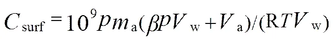
wheresurfstands for concentration of CO in the initial seawater (nmolL−1);is the atmospheric pressure (atm) of dry air;mis the equilibrated headspace mixing ratio (ppbv);is the Bunsen solubility coefficient of CO that varies as a function of temperature and salinity (Wiesenburg and Guinasso, 1979);wis the water sample volume (mL);ais the headspace air volume (mL); R is the gas constant (0.08206atmLmol−1K−1), andis the temperature of seawater (K).

The air-equilibrated seawater CO concentrationeq(nmolL−1) can be calculated using the following equation:

whereatmis the CO mixing ratio of the atmosphere (ppbv); and M is the molar volume of CO at the standard temperature and pressure, 25.094Lmol−1(Lide, 1992; Stubbins., 2006).

The near-instantaneous sea-to-air fluxes of CO were calculated using the following equation:

wherestands for the sea-to-air fluxes of CO (mol m−2h−1);is the gas transfer coefficient (cmh−1) calculated according to the quadratic/wind speed relationship established by Wanninkhof (1992). The coefficientwas adjusted by multiplying (/660)−0.5for the W92 equation. The Schmidt number of CO in the seawater was calculated using the equation of Zafiriou. (2008):

,

whereis in Celsius degrees (℃).

3 Results and Discussion

3.1 Atmospheric CO

The horizontal distribution of atmospheric CO mixing ratios is showed in Fig.2. Atmospheric CO mixing ratio varied from 96 to 256 ppbv with an average of 146 ppbv (SD=54 ppbv,=31) throughout the study area. The highest CO mixing ratio (256ppbv) was observed at coastal station D4-2 and was about 3times higher than the lowest CO mixing ratio (96ppbv) found at open sea station D3-5.Overall, the atmospheric CO mixing ratio displayed a decreasing trend from inshore to offshore stations. Over the southern ECS in this cruise, the concentrations of CO were remarkably higher than their average value for the whole study area. The distributions of CO in the atmosphere showed a gradually decreasing trend from southwest to northeast. The backward trajectory illustrated that air masses originated from adjacent coastal lands and were transported directly to the sampling sites (Fig.3). Thus, the higher CO mixing ratios were probably related to the regionally polluted continental outflow air mass due to the anthropogenic activity.

A similar CO mixing ratio was also obtained by Stubbins. (2006), who reported that the mean CO mixing ratio was 151 ppbv over the ocean from Montevideo, Uruguay (35˚S, 55˚W) to Grimsby, UK (54˚N, 0˚W) in April and May 2000. The average CO mixing ratio in the ECS during November is 238 ppbv (Yang., 2010). According to Lam. (2000), CO mixing ratios in Cape D'Aguilar (22.2˚N, 114.3˚E, 60m above the sea surface) displayed a strong seasonal variation with a maximum in winter and a minimum in summer. The variation trends of CO mixing ratio in the ECS accord with Lam. (2000) results.

3.2 Dissolved CO in Seawater

The CO concentrations obtained from the surface water of the ECS are shown in Fig.4 and the depth, temperature, salinity, time of sampling and wind speed of sampling stations are listed in Table 1. Concentrations of CO in the surface water ranged from 0.24 to 6.12nmolL−1with an average of 1.68nmolL−1(SD=1.50 nmol L−1,=31).

Fig.4 illustrates that the distribution of CO in the surface seawater displayed higher concentrations in the coastal waters and open sea and lower values in the central study area, as also indicated in Fig.5. The higher concentrations of CO (3.35-6.12nmolL−1) were observed at some stations (including stations D1-2, D4-7, D3-1, D2-8, D3-2, D1-3 and D2-7) in the early afternoon (local time 12:00-15:30), mainly due to the high solar radiation. The lower concentrations of CO (0.24 and 0.47nmolL−1) were found at stations D4-1 and D2-1 before dawn (local time 05:40 and 05:24, respectively), which mainly resulted from the lack of solar radiation. The results showed that CO concentrations had good consistency with sampling time, with high values appearing around noon and low values occurring before dawn. This observation suggested that CO distributions were significantly affected by sunlight.

Table 1 The water depth, sampling time (t), surface temperature (T), salinity, and wind speed (u) of sampling stations

Our results are in good agreement with previous studies. For instance, Zafiriou. (2008) found that the surface CO average concentration in the Sargasso Sea was 1.09nmolL−1. However, our results are higher than those obtained in the ECS in November with an average of 0.65nmolL−1(Yang., 2010). This might be attributed to the difference in investigation time. The sunlight photon fluxes of this study in October were obviously higher than those in November (Yang., 2010).

Fig.5 Concentrations of CO and saturation factor in the surface seawater.

Fig.6 Vertical profiles of CO concentrations in the East China Sea.

Fig.7 Diurnal variation of CO concentrations in the surface water.

Four representative vertical profiles of CO concentrations along with the salinity and temperature are shown in Fig.6. It is apparent from Fig.6 that the concentrations of CO in the water column gradually decreased with depth, in agreement with previous studies (Conrad., 1982). The highest concentration of CO was observed in the surface water, which was obviously due to the enhanced photoproduction of CO under the high light intensity. Meanwhile, CO could be detected even at large depths, such as 770 and 1100m, where light intensity was beyond detection limit, indicating the existence of other sources of CO, such as dark production, diffusion, and sediment (Seiler, 1978; Zhang., 2008).

The diurnal variations of CO were investigated at an anchor station D4-3 as shown in Fig.7. Concentrations of CO in the surface seawater exhibited an evident diurnal variation, with the maximal concentration occurring in early afternoon and the minimal concentration appearing before dawn. This variation pattern indicated that the photochemical production of surface CO was driven primarily by light intensity. Jones (1991) also found the similar diurnal variation of CO in seawater and reported that CO concentrations varied by a factor within 2-20 in the diurnal cycle. Our observations are in good agreement with the previous researches (Yang., 2010; Yang., 2011).

3.3 Sea-to-Air Flux of CO

The saturation factors of CO at the investigated sitesare presented in Fig.5. In the present study, the saturation factors varied from 1.4 to 56.9 with an average of 16.8 (SD=15.7,=31). At all investigated sites, the saturation factors were more than 1.00, indicating that CO in the seawater was supersaturated relative to the atmosphere. The mean saturation factor obtained in this study was close to that reported by Zafiriou. (2008) for the Sargasso Sea (mean 18.7), but lower than that of Xie. (2009) for the southeastern Beaufort Sea (mean 45.4 ± 23.4).

Sea-to-air fluxes of CO at the investigated sites are presented in Fig.8. The fluxes ranged from 0.06 to 11.31 μmolm−2d−1with an average of 2.90μmolm−2d−1(SD=2.95μmolm−2d−1,=31). The maximum CO flux appeared at station D1-2 with a considerable saturation factor (35.3) and high wind speed (6.3ms−1). The minimum CO flux occurred at station D4-2 which had a low saturation factor (1.6) and low wind speed (2.5ms−1). Obviously, CO flux is simultaneously influenced by saturation factor and wind speed.

The calculation of CO flux in this study could be used to estimate the contribution of CO from the global coastal area to the CO budget of the global oceans. The coastal zone is the continental shelves to 200m in depth, occupying 7% to 10% of the surface area of the ocean(about30×106km2) (Ver., 1990).Applying our data to the global coastal zone, CO flux was estimated to 0.38 Tg CO-C yr−1. This coastal flux value accounts for 10.3%of the global oceanic emission of CO, assuming the global open ocean emissions of CO to be around 3.7 Tg CO-C yr−1(Stubbins., 2006). Our results showed that the coastal contribution to the global CO emissions should not be ignored.

Fig.8 Relationship between the sea-to-air flux of CO and wind speed in the study area.

3.4 Microbial Consumption Rate of CO

The method of whole-water dark incubation was applied to determine the microbial CO consumption rate constants. Two typical results of microbial CO consumption rate constants are shown in Fig.9. In the incubation experiments, CO concentrations decreased exponentially with incubation time and the processes conformed to the first order reaction characteristics. The2of the fitting for each experiment, rate constant (CO) and biological turnover time (bio) are shown in Table 2. At the stations where incubation experiments were performed, microbial CO consumption rate constant ranged from 0.063 to 0.22 h−1, with an average of 0.12h−1(SD=0.062h−1,=6) (Table 2). Our results were lower than those reported by Xie. (2005) who found thatCOranged from 0.071 to 0.91h−1 in the Northwest Atlantic in summer, with a mean of 0.26h−1. This might be attributed to the difference in seasonal variation. In the present study, the highestCOappeared at station D1-3 with a relatively low salinity and the lowestCOwas observed at station D4-6 which was characterized by the highest salinity.

Fig.9 Typical [CO] versus incubation time at stations D3-3 and D4-6.

Table 2 Microbial CO consumption rate constant (KCO), biological turnover time (τbio) and the regression coefficient (R2) between incubation time and CO concentration

Fig.10 Relationship between KCO and salinity.

The plot ofCOversus the salinity is shown in Fig.10, indicating thatCOvalues decreased linearly with increasing salinity (2=0.67,=6,=0.05). Coastal water salinity was relatively small, indicating that the microbial consumption rate of COin coastal waters was higher than that in the open sea. This result might be due to the more microorganisms in coastal waters (Butler., 1987; Jones and Amador, 1993; Tolli and Taylor, 2005; Najjar., 2003). This trend is consistent with the literature result (Xie., 2005; Yang., 2010) thatCOincreased with the increasing salinity in the range of 0 to 19 but declined with further increasing salinity.COversus the chlorophyllconcentration was also investigated in the present study and there is a poor correlation between them (2=0.45,=6,=0.14) compared with the result of Xie. (2005) (2=0.944). This investigation implies that factors which may influenceCOare very complex in the marine environment and chlorophyllis not a good indicator of CO biological consumption in the ECS during autumn.

4 Conclusions

In the present study, the distribution, flux and biological consumption of CO in the ECS were investigated, and some important conclusions were drawn as follows.

1) Atmospheric CO mixing ratios varied from 96 to 256 ppbv, with an average of 146 ppbv (SD=54 ppbv,=31). Overall, the concentrations of atmospheric CO displayed a decreasing trend from inshore to offshore stations.

2) The surface water CO concentrations in the ECS exhibited a significant spatio-temporal variation. The higher concentration of CO was observed in the daytime, due to the enhanced photoproduction of CO. Vertical profiles showed that CO concentrations declined rapidly with depth, with the maximum value appearing in the surface water.

3) The surface CO concentrations in the ECS in autumn were oversaturated with an average saturation factor of 16.8, indicating that the continental shelf zone was a significant source of atmospheric CO.

4) In the incubation experiments, CO concentrations decreased exponentially with incubation time and the processes conformed to the first order reaction characteristics. The microbial CO consumption rate constants in the surface water (CO) ranged from 0.063 to 0.22h−1with an average of 0.12h−1(SD=0.062h−1,=6). A negative correlation betweenCOand salinity was observed in the present study.

Acknowledgements

The authors are grateful to the captain and crew of the R/V ‘3’ for their help and cooperation during the investigation. This work was financially supported by the National Natural Science Foundation of China (Grant Nos. 40976043 and 41320104008), the National Natural Science Foundation for Creative Research Groups (No. 41221004), the Changjiang Scholars Programme, Ministry of Education of China, and the Taishan Scholars Programme of Shandong Province.

Bates, T. S., Kelly, K. C., Johnson, J. E., and Gammon, R. H., 1995. Regional and seasonal variations in the flux of oceanic carbon monoxide to the atmosphere., 100 (D11): 23093-23101.

Butler, J. H., Jones, R. D., Garber, J. H., and Gordon, L. I., 1987. Seasonal distribution and turnover of reduced trace gas and hydroxylamine in Yaquina Bay, Oregon., 51: 697-706.

Conrad, R., and Seiler, W., 1980. Photo-oxidative production and microbial consumption of carbon-monoxide in seawater., 9 (1): 61-64.

Conrad, R., and Seiler, W., 1982. Utilization of traces of carbon monoxide by aerobic oligotrophic microorganisms in ocean, lake and soil., 132 (1): 41-46.

Conrad, R., Seiler, W., Bunse, G., and Giehl, H., 1982. Carbon monoxide in seawater (Atlantic Ocean)., 87 (C11): 8839-8852.

Erickson III, D. J., 1989. Ocean to atmosphere carbon monoxide flux: global inventory and climate implications., 3: 305-314.

Gammon, R. H., and Kelly, K. C., 1990. Photochemical production of carbon monoxide in surface waters of the Pacific and Indian oceans.In:, Blough, N. V., and Zepp, R. G., eds., Woods Hole Oceanographic Institution, Woods Hole, Mass, 58-60.

Gnanadesikan, A., 1996. Modeling the diurnal cycle of carbon monoxide: sensitivity to physics, chemistry, biology, and optics., 101 (C5): 12177- 12191.

Johnson, J. E., and Bates, T. S., 1996. Sources and sinks of carbon monoxide in the mixed layer of the tropical South Pacific Ocean., 10 (2): 347-359.

Jones, R. D., and Amador, J. A., 1993. Methane and carbon monoxide production, oxidation, and turnover times in the Caribbean Sea as influenced by the Orinoco River., 98: 2353-2359.

Kettle, A. J., 1994. A model of the temporal and spatial distribution of carbon monoxide in the mixed layer. M. Sc. thesis, WHOI/MIT Joint Program, Woods Hole, Mass, 146pp.

Kettle, A. J., 2005. Diurnal cycling of carbon monoxide (CO) in the upper ocean near Bermuda., 8: 337-367.

Khalil, M. A. K., and Rasmussen, R. A., 1990. The global cycle of carbon-monoxide: Trends and mass balance., 20 (1-2): 227-242.

Lam, K. S., Wang, T. J., Chan, L. Y., Wang, T., and Harris, J., 2000. Flow patterns influencing the seasonal behavior of surface ozone and carbon monoxide at a coastal site near Hong Kong., 35: 3121-3135.

Lide, D. R., 1992., CRC Press, Ann Arbor, 12-25.

Lu, X. L., Yang, G. P., Wang, X. M., Wang, W. L., and Ren, C. Y., 2010. Determination of carbon monoxide in seawater by headspace analysis., 38: 352-356.

Najjar, R., Long, R., Zafiriou, O., and Johnson, J., 2003. Impact of physical processes on the diurnal cycle of carbon monoxide. Ocean Science Meeting Supply, Abstract 0532H-IO, EOS Trans. AGU, 1pp.

Ren, C. Y., Yang, G. P., and Lu, X. L., 2014. Autumn photoproduction of carbon monoxide in Jiaozhou Bay, China., 13 (3): 428-436.

Rhee, T. S., 2000.Ph.D. thesis. Texas A and M University, College Station, TX, 23-34.

Seiler, W., 1978. The influence of the biosphere on the atmospheric CO and H2cycles. In:. Krumbein, W. E., ed., Ann Arbor Sci., Ann Arbor, Mich., 773-810.

Stubbins, A., Uher, G., Kitidis, V., Law, C., Upstill-Goddard, R. C., and Woodward, E. M. S., 2006. The open-ocean source of atmospheric carbonmonoxide., 53: 1685-1694.

Su, J. L., 1998. Circulation dynamics of the China seas north of 18˚N. In:,. 11, Robinson, A. R., and Brink. K. H., eds., John Wiley, Hoboken, 483-505.

Thompson, A. M., 1992. The oxidizing capacity of the Earth's atmosphere: Probable past and future changes., 256: 1157-1165.

Tian, R. C., Hu, F. X., and Martin, J. M., 1993. Summer nutrient fronts in the Changjiang (Yangtze River) estuary., 37: 27-41.

Tolli, J. D., and Taylor, C. D., 2005. Biological CO oxidation rates in the Sargasso Sea and in Vineyard Sound, Massachusetts., 50: 1205-1212.

Wanninkhof, R., 1992. Relationships between wind speed and gas exchange over the ocean., 97 (C5): 7373-7382.

Wiesenburg, D. A., and Guinasso, N. L., 1979. Equilibrium solubilities of methane, carbon monoxide and hydrogen in water and sea water., 24: 356-360.

Xie, H., Zafiriou, O. C., Umile, T. P., and Kieber, D. J., 2005. Biological consumption of carbon monoxide in Delaware Bay, NW Atlantic and Beaufort Sea., 290: 1-14.

Xie, H., Belanger, S., Demers, S., Vincent, W. F., and Papakyriakou, T. N., 2009. Photo-biogeochemical cycling of carbon monoxide in the southeastern Beaufort Sea in spring and autumn., 54 (1): 234 -249.

Yang, G. P., Ren, C. Y., Lu, X. L., Liu, C. Y., and Ding, H. B., 2011. Distribution, flux, and photoproduction of carbon monoxide in the East China Sea and Yellow Sea in spring., 116 (C02001), DOI: 10. 1029/2010JC 006300.

Yang, G. P., Wang W. L., Lu X. L., and Ren, C. R., 2010. Distribution, flux and biological consumption of carbon monoxide in the Southern Yellow Sea and the East China Sea., 122: 74-82.

Zafiriou, O. C., Andrews, S. S., and Wang, W., 2003. Concordant estimates of oceanic carbon monoxide source and sink processes in the Pacific yield a balanced global ‘blue-water’ CO budget., 17 (1): 1015- 1027.

Zafiriou, O. C., Xie, H., Nelson, N. B., Najjar, R. G., and Wang, W., 2008. Diel carbon monoxide cycling in the upper Sargasso Sea near Bermuda at the onset of spring and in midsummer., 53: 835-850.

Zhang, J., 1996. Nutrient elements in large Chinese estuaries., 16: 1023-1045.

Zhang, Y., Xie, H., Fichot, C. G., and Chen, G. H., 2008. Dark production of carbon monoxide (CO) from dissolved organic matter in the St. Lawrence estuarine system: Implication for the global coastal and bluewater CO budgets., 113 (C12020), DOI: 10.1029/2008JC 004811.

Zuo, Y., and Jones, R. D., 1995. Formation of carbon-monoxide by photolysis of dissolved marine organic material and its significance in the carbon cycling of the oceans., 82 (10): 472-474.

(Edited by Ji Dechun)

DOI 10.1007/s11802-015-2889-1

ISSN 1672-5182, 2015 14 (6): 994-1002

© Ocean University of China, Science Press and Springer-Verlag Berlin Heidelberg 2015

(January 11, 2015; revised April 19, 2015; accepted May 26, 2015)

* Corresponding author. Tel: 0086-532-66782657 E-mail:gpyang@mail.ouc.edu.cn