Study on the dependence of the two-dimensional Ikeda model on the parameter

LI Qing， ZHENG Qin，bnd ZHOU Shi-Zheng

aCollege of Science， PLA University of Science and Technology， Nanjing 211101， China；bState Key Laboratory of Numerical Modeling for Atmospheric Sciences and Geophysical Fluid Dynamics， Institute of Atmospheric Physics， Chinese Academy of Sciences， Beijing 100029， China

Study on the dependence of the two-dimensional Ikeda model on the parameter

LI Qianga， ZHENG Qina，band ZHOU Shi-Zhenga

aCollege of Science， PLA University of Science and Technology， Nanjing 211101， China；bState Key Laboratory of Numerical Modeling for Atmospheric Sciences and Geophysical Fluid Dynamics， Institute of Atmospheric Physics， Chinese Academy of Sciences， Beijing 100029， China

Based on the property of solutions of the nonlinear differential equation， this paper focuses on the behavior of solutions to the two-dimensional Ikeda model， especially the dependence of the solutions on the parameter. The dependency relationship of the two-dimensional Ikeda model on the parameter is revealed by a large sample of proper numerical simulations. With the parameter varying from 0 to 1， the numerical solutions change from a point attractor to periodic solutions， then to chaos， and end up with a limit cycle. Furthermore， the route from bifurcation to chaos is shown to be continuous period-doubling bifurcations. The nonlinear structures presented by the solution of the two-dimensional Ikeda model indicate that， by setting different model parameters， one can test a new method that will be adopted to study atmospheric or oceanic predictability and/or stability. The corresponding test results provide some useful information on the ability of the new approach overcoming the impacts of strong nonlinearity.

ARTICLE HISTORY

Ikeda model； attractor；chaos； bifurcation

中文题名：探究二维Ikeda模式解对参数的依赖

研究目的：探索二维Ikeda模式数值解的性态及解对模式参数的依赖

创新要点：首次对二维Ikeda模式解的性态进行全面细致的探究；结合非线性方程相关理论和数值试验结果给出解的分析；探究了各个分岔点大致的分岔值。

研究方法：数值试验与理论分析相结合

重要结论：二维Ikeda模式对于控制参数具有高度依赖性；参数值从0到1的变化过程中，模式经历了从单点吸引子、多点吸引子、产生混沌直至出现极限环的变化；模式通过倍周期分岔的方式从分岔到混沌，且分岔过程是连续的。

Introduction

To forecast a weather phenomenon or an ocean event， due to the effect of nonlinearity， the predictability of the phenomenon or event should be the first concern. A natural idea is to study practical dynamic models directly. However，considering the complexity of practical models， including high dimensionality and the complex interactions of the practical situation， this paper utilizes a simple idealized model， which can depict some important dynamic processes of the practical model， such as the nonlinear process to investigate the theory of， and methods for， predictability issues， and then apply the result to research on practical forecasting models （Mu and Duan 2003）.

Actually， the Lorenz model has been used as an idealized model in forecast research， not only for its simplicity and strong nonlinearity， but also for its comprehensive analysis of the property and stability of the solution. Some results from predictability studies based on the Lorenz model have been applied to help predict practical situations （Ding and Li 2012； Zheng et al. 2012）.

The Ikeda model was originally proposed by Kensuke Ikeda as a model of light going across a nonlinear optical resonator （ring cavity containing a nonlinear dielectric medium）， and the two-dimensional Ikeda difference scheme is its most common form. As a nonlinear dynamic system model， the Ikeda model is less popular compared with the Lorenz model， despite being stronger.

Owing to the interactions of nonlinearity， characters including attractors， saddle points， and chaos usually appear in different regions of nonlinear dynamic systems. An attractor， which exists in the phase plane， is an important concept in dynamics， used to describe the convergent features of movement. In short， an attractor is a set to which every point or orbit nearby converges （Xi and Xi 2007）. An attractor can be in different forms， such as a fixed point， a limit cycle， an integer-dimension torus， and a singular one. A saddle point is a singular point that is stable along a certain direction， but unstable along another （Fu and Fan 2011）. The chaotic phenomenon， referring to a certain but unpredictable movement， is currently a keyissue in nonlinear dynamics. It shows randomness， but is definitely a stochastic-like process from a deterministic system （Niu 2007）. Chaos is commonly bifurcated by the fixed point， such as period-doubling bifurcation， fits-bifurcation，hysteresis， and elusive saltation and bifurcation controlled by double parameters. It is chaos that allowed Lorenz to propose the predictability issue for atmospheric motion.

Stemler and Judd （2009） applied the shadowing filter method to state estimation， preliminary data assimilation，and predictability research in the two-dimensional Ikeda model. In their numerical experiment， the parameter of the Ikeda model was set to a fixed value， and relevant analysis only focused on limited initial values. The result of the numerical experiment in Stemler and Judd （2009） indicates that the system develops to chaos just right with the parameter they selected， so the applicability of their method for other situations needs further exploration. Chen， Chen， and Ma（1990） analyzed the Ikeda instability of optical bistability and derived the Ikeda equation in another way， revealing the physical origin of the instability of optical bistability. However， they focused only on the physical origin of the Ikeda model， without further discussion of the solution of the model. Xie and Zhang （2007） investigated the adaptive synchronization of the Ikeda system and demonstrated the effectiveness of this method， without analyzing the Ikeda model. Chui et al. （2004） used Ikeda time series with variable parameters to verify the effectiveness of the support vector machine model they established in their article and noticed that the solutions of the two-dimensional Ikeda model change with the variation of the parameter. However， their aim was to predict with the model instead of discussing the dependence of the model on the parameter.

Many scholars have worked on the two-dimensional Ikeda model since it was proposed （Chen， Chen， and Ma 1990； Chui et al. 2004； Liu 2009； Stemler and Judd 2009； Xie and Zhang 2007）， but in most cases they used the model to study the issue of concern， without comprehensive and detailed discussion about the behavior of the model solution. Usually， one only uses the Ikeda model with a specific model parameter and initial condition to test the effectiveness of a new method in terms of the estimation of the model state， predictability and data assimilation（Chui et al. 2004； Stemler and Judd 2009； Xie and Zhang 2007）. The present study attempts to comprehensively investigate the behavior of the Ikeda model solution by using the theory of nonlinear dynamic systems.

The two-dimensional Ikeda model has stronger nonlinearity than the Lorenz model. Therefore， it can be an alternative to the Lorenz model when testing the ability of a new approach for overcoming the impacts of strong nonlinearity. In order to use this model more effectively，it is necessary to know the characteristics of the nonlinear interactions， such as attractors， saddle points， and the chaos demonstrated by the model solution. This is the objective of the present study. Based on the behavior and stability of the nonlinear differential equation solutions，this study aims to investigate the two-dimensional Ikeda model solution's behavior， and reveal the dependency of the solution on the model parameter by numerical experiments.

The two-dimensional Ikeda model

The Ikeda model is a series of delay differential equations，proposed by Kensuke Ikeda when he explored the nonlinear dielectric medium. Deduced through the Maxwell-Bloch equations （Ikeda 1979）， it can be simplified as difference equations， as shown below:

Here， i is the imaginary unit； t represents the time step； z stands for the electric field inside the ring cavity； and A， B，C are physical parameters. A is related to the intensity of the incident light and indicates laser light applied from the outside； B is called the dissipation parameter， characterizing the dissipation of the electric field； and C indicates the laser light applied from the outside. A two-dimensional case of Equation（1） is the common two-dimensional Ikeda model:

In Equation （2）， the value range of the parameter μ is［0， 1］， and

The values of a and b are usually 0.4 and 6， respectively. From the expression of the model we find that the trigonometric functions appear in Equation （2）， and Equation（3） is a fraction whose denominator includes two quadratic components. Clearly， the two-dimensional Ikeda model has fairly strong nonlinearity， which means the solutions of the model will experience a fair amount of movement with the variation of the parameter.

Behavior of the solutions and the dependence on the parameters of the model

For the two-dimensional Ikeda model， Equation （2）， it seems it is difficult to obtain the corresponding analytical solutions directly. Therefore， through a large sample of numerical experiments， this paper attempts to achieve a comprehensive and more accurate understanding of thebehavior of its solutions， to reveal the dependence of the model on the parameter.

Figure 1.Solutions of the last 5000 steps when the model parameter μ = 0.402 and 0.403.

Figure 2.Solutions of the last 5000 steps when μ = 0.500， 0.600， and 0.640.

Figure 3.Solutions of the last 5000 steps when μ = 0.643， 0.644， and 0.650.

Figure 4.Solutions of the last 5000 steps when μ = 0.902 and 1.000.

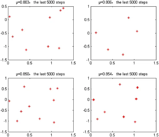
Figure 5.Elusive saltation in a chaotic situation （solutions of the last 5000 steps are shown here when μ = 0.803， 0.806， 0.850， and 0.854t）.

To explore the influence of different parameter values on the behavior of the model solutions， the internal ［0， 1］ is equally divided into 1000 segments and the value of every 1/1000 equant point is assigned to the model parameter μ. The initial value chosen in this paper is （x0， y0） = （0.25， -0.325）. For every value of the parameter， the model is integrated 10，000 steps along with time. This paper chooses and analyzes several representative situations， the results of which are shown in Figures 1-6. A more comprehensive statistical result of the numerical tests is given in Table 1. Since the observation of attractors may be affected by the irregular trajectory of points before the model reaches a plateau， in this paper the first five figures only show results of the last 5000 steps，when the model becomes stable.

Figure 6.Behavior of solutions from chaos to a limit cycle （solutions are shown here when μ = 0.903， 0.950， 0.990， and 0.999）.

Table 1.The relationship between solutions and the parameter.

Figure 1 shows the result of the last 5000 steps when the parameter μ = 0.402 and 0.403. The abscissa and the ordinate represent two components of the state in the model （the same in subsequent figures）. The result shows that when the value of μ is set between 0 and 0.402， the model solutions will evolve to one point after a certain period. That is to say， the system has a point attractor on this occasion. The number of the convergence point increases when the value of μ is equal to or greater than 0.403. In Figure 1， when μ varies from 0.402 to 0.403， the system changes from a point attractor to a periodic solution with a cycle of 2. Clearly， a bifurcation exists between 0.402 and 0.403， and the critical value of the parameter，namely the bifurcation value， is between the two values of μ.

Comparing the three sub-graphs of Figure 2， along with the variation of μ from 0.500 to 0.600 the model experiences a bifurcation from two convergence points to four， which means the cycle of the periodic solution changes from two to four. Analogously， the cycle of the solution turns into eight from four as μ varies from 0.600 to 0.640.

From Figure 3 it can be clearly seen that the cycle of the solutions changes from eight to sixteen as the value of μ changes from 0.643 to 0.644. When μ continues to increase to 0.650， the system will lose its periodic solution.

As shown in Figure 4， when μ = 0.900， obvious chaos appears in the system； and when μ = 1.000， the system presents a limit cycle. Results also show that the system gradually develops towards chaos when the value of μ varies from 0.646 to 0.700. As the value of μ varies from 0.700 to 0.902， the system has apparent chaos. Elusive saltationin chaotic cases occurs when the value of μ varies from 0.803 to 0.808， μ = 0.850 and 0.854， as shown in Figure 5.

Meanwhile， with variation of μ from 0.903 to 0.999， the system presents chaos at first， and then breaks away from chaos until a singular attractor appears in a new region（shown in Figure 6）.

Combining the numerical test results with Figures 1-6，and consulting the theory of the behavior and the stability of the nonlinear differential equation solution， we obtain the relationship between the behavior of the two-dimensional Ikeda model solutions and the model parameter μ，as shown in Table 1.

Conclusion

From the numerical experiment described in this paper we find that the solutions of the model change with the variation of the parameter. Moreover， small parametric variation may result in great differences of solutions in certain ranges. The conclusion above reflects the high dependence of the two-dimensional Ikeda model on the parameter. Specifically， when the parameter varies from 0 to 1， the numerical solutions change from a point attractor to periodic solutions， then to chaos， and finally become a limit cycle. According to the bifurcation theory of the behavior and stability of the nonlinear differential equation solutions， we conclude that the varying process of the solutions of the two-dimensional Ikeda model along with the variation of the parameter is actually a course from bifurcation to chaos through continuous period-doubling bifurcations. With the increase of the model parameter μ， the numerical solutions of this model possess a range of nonlinear behavior， which perfectly corresponds to analyses of nonlinear theory. Its nonlinear characteristics presented by the movement from bifurcation to chaos make the model an alternative to the Lorenz model. In view of the results of this study，one can choose a special model parameter to verify the effectiveness of an estimation method for different characteristic solutions of the two-dimensional Ikeda model. Since the Ikeda model has stronger nonlinearity than the Lorenz model， it is more significant to study predictability problems based on the Ikeda model. Also， we can use the Ikeda model to explore the influence of model parameter error on data assimilation according to the critical parameter values obtained in this paper. In addition， both the accuracy of the bifurcation values and the transition of the model from chaos to a limit cycle deserve further research in the future.

Funding

This work was supported by the National Natural Science Foundation of China ［grant number 41331174］.

References

Chen， L. X.， J. S. Chen， and A. Q. Ma. 1990. “Instability Analysis of Optical Bistability in Ring Cavity and the Physical Origin of the Ikeda Instability.” Journal of Natural Science of Heilongjiang University 7 （4）: 59-64.

Chui， W. Z.， C. C. Zhu， W. X. Bao， and J. H. Liu. 2004. “Prediction of the Chaotic Time Series Using Support Vector Machines.” Acta Physica Sinica 53 （10）: 3303-3310.

Ding， R. Q.， and J. P. Li. 2012. “Relationships between the Limit of Predictability and Initial Error in the Uncoupled and Coupled Lorenz Models.” EGU General Assembly 2013 29 （5）: 1078-1088. Fu， X. L.， and J. J. Fan. 2011. Nonlinear Differential Equation. Beijing: Science Press.

Ikeda， K. 1979. “Multiple-valued Stationary State and Its Instability of the Transmitted Light by a Ring Cavity System.”Optics Communications 30 （2）: 257-261.

Liu， Z. Z. 2009. “Non-resnonant Double Hopf Bifurcation in an Ikeda Model and a Van Der Pol-Duffing Oseillator with Time Delay.” M.S.'s thesis， Zhengzhou University.

Mu， M.， and W. S. Duan. 2003. “A New Approach to Studying ENSO Predictability: Conditional Nonlinear Optimal Perturbation.”Chinese Science Bulletin 48 （10）: 1045-1047.

Niu， H. 2007. “Stability Analysis of Nonlinear Differential Equations.” M.S.'s thesis， Liaoning University of Technology.

Stemler， T.， and K. Judd. 2009. “A Guide to Using Shadowing Filters for Forecasting and State Estimation.” Physica D: Nonlinear Phenomena 238 （14）: 1260-1273.

Xi， D. X.， and Q. Xi. 2007. Nonlinear Physics. Nanjing: Nanjing University Press.

Xie， Y. H.， and H. G. Zhang. 2007. “Adaptive Synchronization for a Class of Delayed Ikeda Chaotic Systems.” Journal of Northeastern University （Natural Science） 28 （4）: 481-484.

Zheng， Q.， Y. Dai， L. Zhang， J. X. Sha， and X. Q. Lu. 2012. “On the Application of Genetic Algorithm to the Predictability Problems Involving “on-off” Switches.” Advances in Atmospheric Sciences 29 （2）: 422-434.

组

Ikeda模式； 吸引子； 混沌； 分岔

9 April 2015 Accepted 6 July 2015

CONTACT ZHENG Qin qinzheng@mail.iap.ac.cn

© 2016 The Author（s）. Published by Taylor & Francis

This is an Open Access article distributed under the terms of the Creative Commons Attribution License （http://creativecommons.org/licenses/by/4.0/）， which permits unrestricted use，distribution， and reproduction in any medium， provided the original work is properly cited.