Unrealistic treatment of detrained water substance in FGOALS-s2 and its influence on the model's climate sensitivity

HE Bian

aState Key Laboratory of Numerical Modeling for Atmospheric Sciences and Geophysical Fluid Dynamics， Institute of Atmospheric Physics，Chinese Academy of Sciences， Beijing 100029， China；bKey Laboratory of Meteorological Disaster of Ministry of Education， Nanjing University of Information Science and Technology， Nanjing 210044， China

Unrealistic treatment of detrained water substance in FGOALS-s2 and its influence on the model's climate sensitivity

HE Biana，b

aState Key Laboratory of Numerical Modeling for Atmospheric Sciences and Geophysical Fluid Dynamics， Institute of Atmospheric Physics，Chinese Academy of Sciences， Beijing 100029， China；bKey Laboratory of Meteorological Disaster of Ministry of Education， Nanjing University of Information Science and Technology， Nanjing 210044， China

Based on a series of aqua-planet and air-sea coupled experiments， the influence of unrealistic treatment of water substance in the Flexible Global Ocean-Atmosphere-Land System Model，spectral version 2 （FGOALS-s2）， on the model's climate sensitivity is investigated in this paper. Because the model does not adopt an explicit microphysics scheme， the detrained water substance from the convection scheme is converted back to the humidity. This procedure could lead to an additional increase of water vapor in the atmosphere， which could strengthen the model's climate sensitivity. Further sensitivity experiments confirm this deduction. After removing the water vapor converted from the detrained water substance， the water vapor reduced significantly in the upper troposphere and the high clouds also reduced. Quantitative calculations show that the water vapor reduced almost 10% of the total water vapor， and 50% at 150 hPa， when the detrained water substance was removed， contributing to the 30% atmospheric surface temperature increase. This study calls for an explicit microphysics scheme to be introduced into the model in order to handle the detrained water vapor and thus improve the model's simulation skill.

ARTICLE HISTORY

FGOALS-s2； climate

sensitivity； cloud radiation；global warming

在CMIP5的历史情景试验中，FGOALS-s2模拟的地表温度趋势远大于观测和其他气候系统模式，表现出较高的气候敏感性。本文通过一系列水球试验和海气耦合试验，研究了FGOALS-s2大气分量模式对流-辐射过程中对流参数化卷出云水云冰的处理问题，发现了模式诊断出的次网格尺度的云水云冰辐射效应过强，导致热带地区对流层高层水汽反馈和长波云辐射反馈过程偏强，是模式高敏感性的主要原因。文章强调了需要引入显式的云微物理过程来克服这种不确定性。

1. Introduction

Cloud formation processes span scales from the sub-micrometer scale of cloud condensation nuclei， to cloud systems of up to thousands of kilometers. This range of scales is impossible to resolve in climate models （IPCC 2013）， and various clouds schemes are applied to simulate the cloud macro- and micro-properties and the associated radiative forcings. Despite decades of advancement， cloud parameterization schemes， especially microphysics schemes，still contain many uncertainties， which lead to the largest uncertainty in simulating cloud feedbacks and to a wide range of climate sensitivity in state-of-the-art climate models （Wang et al. 1976； Hall and Manabe 1999； Kristin et al. 1999； Schneider et al. 1999； Gettelman et al. 2012）.

The Flexible Global Ocean-Atmosphere-Land System Model， spectral version 2 （FGOALS-s2）， is a climate system model developed at the State Key Laboratory of Numerical Modeling for Atmospheric Sciences and Geophysical Fluid Dynamics， Institute of Atmospheric Physics （LASG/IAP）（Bao et al. 2010， 2013） in which the atmospheric model Spectral Atmosphere Model developed at LASG/IAP， version 2 （SAMIL2） is applied. SAMIL2 uses a diagnostic method to estimate the effective radius of cloud droplets for both the liquid and ice phase， which is based on the detrained liquid water content in the convection scheme and assumed droplet concentrations in the cloud （Martin et al. 1994）. Because the model does not employ an explicit microphysics scheme to simulate cloud condensation nuclei and the associated radiative forcings， the detrained water substance （cloud water and cloud ice） in the convection scheme is evaporated back to the water vapor in the atmosphere after deep convection occurs. This treatment will potentially cause excessive water vapor in the upper troposphere and lead to an excessively strong water vapor feedback and high climate sensitivity.

Recently， two studies （Zhou et al. 2013； Chen et al. 2014）have revealed that FGOALS-s2 shows quite high climate sensitivity in response to increasing greenhouse gases（GHGs） in both historical simulations and future projections， which may be related to the excessively strong water vapor feedback in the model. Whether or not the unrealistic treatment of converting detrained water substance to the water vapor is related to the model's high climate sensitivity remains unclear. Therefore， in this study， based on a series of aqua-planet experiments and an air-sea coupled experiment， the influence of the unrealistic treatment of detrained water vapor in SAMIL2 on the radiation forcing is investigated. The contribution of the unrealistic treatment to the model's high climate sensitivity is measured quantitatively. Additionally， an eventual solution to the high climate sensitivity of FGOALS-s2 is also discussed. The remainder of the paper is organized as follows: Section 2 introduces the datasets， the model configurations， and the experimental design. Section 3 reports the results. Section 4 presents the final conclusions and a discussion.

2. Datasets and model configuration

2.1. Datasets

The Goddard Institute for Space Studies （GISS） Surface Temperature Analysis dataset is used for observation in the present study （Hansen et al. 2010）. This dataset is on a 2° × 2° grid and covers the period 1880 to the present day with monthly mean anomalies. More details of the documentation of the datasets can be found at http://data.giss.nasa.gov/ gistemp/.

The monthly mean outputs of atmospheric surface temperature （AST） of 24 CMIP5 （Coupled Model Intercomparison Project Phase 5） climate models （ACCESS1-0， BCC-CSM1-1，CanESM2， CCSM4， CESM1-CAM5， CMCC-CM， CNRM-CM5，CSIRO-Mk3-6-0， EC-EARTH， FGOALS-g2， GFDL-CM3， GFDLESM2G， GISS-E2-H， GISS-E2-R， HadGEM2-AO， HadGEM2-ES，INMCM4， IPSL-CM5A-LR， MIROC5， MIROC-ESM， MPI-ESM-LR，MPI-ESM-MR， MRI-CGCM3， and NorESM1_M） are used to obtain the multi-model ensemble （MME）. The datasets covers the period from 1880 to 2005 and are derived from the website http://pcmdi9.llnl.gov/esgf-web-fe/.

2.2. Model configuration

The climate system model FGOALS-s2 is composed of four individual components: SAMIL2 （Wu et al. 1996； Bao et al. 2010）； version 2 of the LASG/IAP Climate System Ocean Model， LICOM2 （Liu et al. 2013）； version 3 of the Community Land Model， CLM3 （Oleson et al. 2004）； and version 5 of the Community Sea Ice Model， CSIM5 （Briegleb et al. 2004）. The exchanged fluxes among these components are connected by the National Center for Atmospheric Research（NCAR） coupler module 6 （Collins et al. 2006）. The basic performances of the models are described in Bao et al.（2013）.

The atmospheric model SAMIL2 has an R42 horizontal resolution （2.81° longitude × 1.66° latitude） with 26 vertical layers in a σ-p hybrid coordinate， extending from the surface to 2.19 hPa. The mass flux cumulus parameterization of Tiedtke （1989） is used to calculate convective precipitation. The cloud scheme is a diagnostic method based on relative humidity （RH）， vertical velocity， atmospheric stability， and the convective mass flux associated with parameterized moist convection （Slingo 1987； Kiehl et al. 1996）， while a statistic low cloud method is also applied（Dai et al. 2004）. A nonlocal scheme is employed in the boundary layer to calculate the eddy-diffusivity profile and turbulent velocity scale， and the model incorporates nonlocal transport effects for heat and moisture （Holtslag and Boville 1993）. The radiation scheme employed is an updated Edwards-Slingo scheme （Edwards and Slingo 1996； Sun and Rikus 1999）.

2.3. Experimental design

To investigate the possible influence of the unrealistic treatment of detrained water substance on the model's climate sensitivity， a series of sensitivity experiments were designed， as summarized in Table 1. For simplicity，the detrained water substance in the convection scheme is defined as Δqcl. An aqua-planet control run was performed first， with the default SAMIL2 physics configuration（CON_A） and with the sea surface temperature （SST） forced as in Equation （1）:

Table 1.Experimental design.

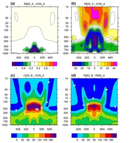
Figure 1.（a） Cross section of water vapor difference （units: g kg-1） between RMQ_A and CON_A. （b） As in （a） but for the water vapor percentage （units: %）. （c） Cross section of water vapor percentage change （units: %） between CON_B and CON_A， and （d） between RMQ_B minus RMQ_A.

whereλdenotes the longitude and ϕ denotes the latitude. The Maximum SST was 27 °C at the equator. Poleward of both 60°N and 60°S the SST remained at 0 °C with sea-ice switched off. More details of the experimental settings can be found in Neale and Hoskins （2001）. The sensitivity run named RMQ_A removed the Δqclin the model's physics but kept other forcings the same as in CON_A. The influences of theΔqclon the model's climate sensitivity were investigated by conducting additional experiments，CON_B and RMQ_B， which were the same as CON_A and RMQ_A， respectively， but a uniform 4 °C addition on the SST for the perturbation. Thus， quantitative measurement of the model's climate sensitivity parameter could be calculated from Equation （2）. Lastly， the possible influence ofΔqclon the evolution of AST in the fully coupled model FGOALS-s2 was estimated. The historical run （CON_CP）was performed from 1850 to 2005， while a sensitivity run（RMP_CP） was performed with the same configuration as CON_CP but with Δqclremoved from the model's physical package.

3. Results

The influence of detrained water substance in the convection scheme on the total water vapor simulation in the model is first examined. The water vapor differences between RMQ_A and CON_A for the mass ratio unit are shown in Figure 1a， and for the percentage in Figure 1b. It is clear that once the Δqclhas been removed the water vapor decreases significantly throughout the troposphere，especially in the tropics （Figure 1a）. Because the radiative effect of absorption by water vapor is roughly proportional to the logarithm of its concentration （IPCC 2013），the change of water vapor in percentage terms is shownin Figure 1b， revealing that the water vapor percentage decreases significantly in the upper troposphere， which would weaken the greenhouse effect from water vapor（Yang and Tung 1998； Minschwaner and Dessler 2004）.

Figure 2.Zonal mean value of （a） clear-sky outgoing longwave radiation （units: W m-2）， （b） 150 hPa relative humidity （units: %）， （c）500 hPa vertical velocity （units: 100 × Pa s-1）， （d） high cloud fraction （units: %）， （e） longwave cloud radiation forcing （units: W m-2）， and（f） shortwave cloud radiation forcing （units: W m-2）， in the four aqua-planet experiments.

Next the change in the vertical water vapor percentage is examined under the uniform +4 °C warming by comparing CON_B minus CON_A and RMQ_B minus RMQ_A （Figures 1c and 1d）. When the increase in upper tropospheric water vapor still contains the amount ofΔ qcl（Figure 1c）， the ratio of the increase of water vapor shows a maximum over the tropics at 100-200 hPa， which exceeds 180%. However， when the Δqclis removed in the second group （RMQ_B minus RMQ_A）， the simulated water vapor change in the upper troposphere weakens significantly（Figure 1d）. The percentage of increased water vapor in the upper troposphere reduces to 150% over the tropics， while remaining almost unchanged at other latitudes. The results of the global mean water vapor change and the vertical distribution indicate that the Δqclaccounts for about 10% of the total water vapor and is more sensitive in the upper troposphere where the convection occurs.

Because the water vapor decreases significantly in the upper troposphere， its own radiative forcing and the associated cloud radiation forcing （CRF） will both change. These two kinds of radiative forcing changes are estimated in the following paragraph. The longwave CRF （LWCRF） is defined as the difference between clear-sky net upward longwave flux and upward longwave flux at the top of the atmosphere （TOA）. The shortwave CRF （SWCRF） is defined as the difference between net downward shortwave fluxes and clear-sky net downward shortwave fluxes.

Because the GHGs are all prescribed in the model，except the water vapor， the change of the clear-sky longwave radiation （LWCS） is mainly induced by the changes of water vapor. It shows clearly that LWCS increases significantly when Δqclis removed （Figure 2a）， and the difference of LWCS between CON_B and RMQ_B is larger when the surface is warming.

The zonal mean RH at 150 hPa is shown in Figure 2b，revealing clearly that the RH decreases from about 80% in CON_A and CON_B to 50% in RMQ_A and RMQ_B. Because the model diagnoses the cloud fraction based on the air temperature and RH （Kiehl et al. 1996）， Figure 2b also indicates that the removal of the radiative effect fromΔqclwill largely reduce the generation of the high cloud fraction in the convective regions， as shown in Figure 2d， while the vertical ascending motion does not change （Figure 2c）. Consequently， the LWCRF （Figure 2e） reduces significantly by about 10 W m-2in the tropics， where convection mainly occurs， while it changes little at other latitudes. This is quite different with the changes in SWCRF （Figure 2f）.

The combined radiative effect of theΔqclon the climate sensitivity can be quantitatively measured by calculating the climate sensitivity parameter. Following Cess et al. （1990）， the climate sensitivity parameterλcan be expressed as

where F and Q denote the global-mean emitted infrared and net downward solar fluxes at the TOA. Thus， ΔF and ΔQ represent the climate change TOA responses to the direct radiative forcing， which are impacted by climate feedback mechanisms.ΔTsdenotes the change in global-mean surface temperature.

In the aqua-planet experiments， the change of surface temperature was equal to 4 °C in both CON_B minus CON_A （CON group） and RMQ_B minus RMQ_A （RMQ group）. Therefore，λis determined by the change in the denominator on the right side of Equation （2）. Equation （2）was calculated in both the CON and RMQ group， revealing λto be 0.65 °C m2W-1in CON and 0.44 °C m2W-1in RMQ.Compared to the results of Cess et al. （1990）， in which a typicalλvalue of 0.5 °C m2W-1was shown， theλfor the CON group is too high. However， when theΔqclis removed in the model's physical package， theλshows a reasonable value that is close to Cess et al. （1990）， indicating a reduction in the model's climate sensitivity. Therefore， from the aqua-planet sensitivity experiments， it is revealed that if the detrained water substance is converted back to water vapor， it can strengthen the water vapor feedback to increase the model's climate sensitivity.

Lastly， the possible influence of Δqclon the evolution of AST is measured directly in the fully coupled model FGOALS-s2. The historical run （named RMQ_CP） was repeated in the same way as CON_CP （Table 1） but with the Δqclremoved from the model's physical package. The linear trends in the vertical water vapor percentage from 1880 to 2005 for CON_CP and RMQ_CP are shown in Figures 3a and 3b， respectively. The ratio of increased water vapor in the upper troposphere reduces to 20-25% in RMQ_CP（Figure 3b）， less than CON_CP （Figure 3a） in which the ratio of increased water vapor is up to 40%. The trend in the absolute amount of water vapor at 150 hPa is 0.63 ppm/126 yr in RMQ_CP， reduced from 1.29 ppm/126 yr in CON_CP. The results indicate that the positive bias of water vapor in the upper troposphere is largely suppressed by removing Δqcl. It also indicates that the greenhouse effect due to water vapor is reduced in RMQ_CP， which will lead to a more realistic simulation in the evolution of global AST.

Figure 3c shows the time series of the annual mean global AST evolution from 1880 to 2005 simulated by CON_CP， RMQ_CP， and the MME， and that observed. After reducing the Δqclin each model step， the evolution of global AST in RMQ_CP is lower than CON_CP and closer to the MME's results. The linear trend of AST during 1880 to 2005 is 1.32 °C/126 yr in RMQ_CP； compared to the 1.79 °C/126 yr in CON_CP， RMQ_CP reduces 30% of the global warming trend. Note that this linear trend is still larger than the MME value of 0.91 °C/126 yr and the observed value of 0.66 °C/126 yr， which demonstrates that the unrealistic treatment of the water substance in the model physics is not the only source of the model's high climate sensitivity. Other possible reasons are to be studied further.

4. Summary and discussion

This study investigates the influence of the unrealistic treatment of detrained water substance in SAMIL2 on the model's climate sensitivity， by carrying out a series of sensitivity experiments. Because the model does not adopt an explicit microphysics scheme， the detrained water vapor from the convection is converted back to the humidity. This procedure leads to an additional increase of water vapor in the upper troposphere， which could strengthen the model's climate sensitivity. Further sensitivity experiments show that the unrealistic treatment increases the water vapor content in the upper troposphere， leading to more high cloud and thus causing an increase in the cloud longwave radiative forcing. Quantitative calculations show that， after removing the detrained water substance in the model's physics， the climate sensitivity parameterλ reduces from 0.65 to 0.44 °C m2W-1. In the historical simulation， the water vapor reduces by almost 50% at 150 hPa when the detrained water substance is removed， contributing to the 30% AST increase.

The present study suggests that it is necessary to implement a physical-based microphysics scheme in SAMIL2. This will mean that the detrained water substance can be directly handled， which is conducive to reducing the model's high climate sensitivity. In fact， the accurate treatment of clouds and their radiative properties should be widely considered as one of the most important issues facing global climate modeling （Hack 1998）. While some of the changes in cloud， cloud water， cloud ice， and cloud distribution provide positive feedback， others provide negative feedback. Therefore， improving radiative effects of the cloud properties in FGOALS-s2 should be the primary approach to improving the model's simulation skill in the future.

Acknowledgments

The author would like to thank the anonymous reviewers for their constructive suggestions， which were indispensable for the improvement of the manuscript.

Funding

This work was jointly supported by the National Basic Research Program of China ［grant number 2014CB953904］， the National Natural Science Foundation of China ［grant numbers 41405091 and 91337110］， the Open Projects of the Key Laboratory of Meteorological Disaster of the Ministry of Education ［grant number KLME1405］， and the Strategic Leading Science Projects of the Chinese Academy of Sciences ［grant number XDA11010402］.

References

Bao， Q.， P. F. Lin， T. J. Zhou， Y. M. Liu， Y. Q. Yu， G. X. Wu， B. He， et al. 2013. “The Flexible Global Ocean-Atmosphere-Land System Model， Spectral Version 2: FGOALS-s2.” Advances in Atmospheric Sciences 30: 561-576.

Bao， Q.， G. X. Wu， Y. M. Liu， J. Yang， Z. Z. Wang， and T. J. Zhou. 2010. “An Introduction to the Coupled Model FGOALS1.1-s and Its Performance in East Asia.” Advances in Atmospheric Sciences 27: 1131-1142. doi:10.1007/s00376-010-9177-1.

Briegleb， B. P.， W. H. Lipscomb， M. M. Holland， J. L. Schramm， R. E. Moritz. 2004. Scientific Description of the Sea Ice Component in the Community Climate System Model， Version Three. NCAR Tech. Note NCAR/TN-463+STR， 70pp.

Cess， R. D.， G. L. Potter， J. P. Blanchet， G. J. Boer， A. D. Del Genio，M. Deque， V. Dymnikov， et al. 1990. “Intercomparison and Interpretation of Climate Feedback Processes in 19 Atmospheric General Circulation Models.” Journal of Geophysical Research 10 （16）: 601-615.

Chen， X. L.， T. J. Zhou， and Z. Guo. 2014. “Climate Sensitivities of Two Versions of FGOALS Model to Idealized Radiative Forcing.” Science China Earth Sciences 57 （6）: 1363-1373.

Collins， W. D.， C. M. Bitz， M. L. Blackmon， G. B. Bonan， C. S. Bretherton， J. A. Carton， P. Chang， et al. 2006. “The Community Climate System Model Version 3 （CCSM3）.” Journal of Climate 19: 2122-2143.

Dai， F. S.， R. C. Yu， X. H. Zhang， Y. Q. Yu. 2004. “A Statistical Lowlevel Cloud Scheme and its Tentative Application in a General Circulation Model.” Acta Meteorologica Sinica 62 （4）: 385-394（in Chinese）.

Edwards， J. M.， and A. Slingo. 1996. “Studies with a Flexible New Radiation Code. I: Choosing a Configuration for a Large-scale Model.” Quarterly Journal of the Royal Meteorological Society 122: 689-719.

Gettelman， A.， J. E. Kay， and K. M. Shell. 2012. “The Evolution of Climate Sensitivity and Climate Feedbacks in the Community Atmosphere Model.” Journal of Climate 25 （5）: 1453-1469.

Hack， J. J. 1998. “Sensitivity of the Simulated Climate to a Diagnostic Formulation for Cloud Liquid Water.” Journal of Climate 11: 1497-1515.

Hall， A. M.， and S. Manabe. 1999. “The Role of Water Vapor Feedback in Unperturbed Climate Variability and Global Warming.” Journal of Climate 12: 2327-2346.

Hansen， J.， R. Ruedy， M. Sato， and K. Lo. 2010. “Global Surface Temperature Change.” Reviews of Geophysics. 48 （4）: RG4004. doi:10.1029/2010RG000345.

Holtslag， A. A. M.， and B. A. Boville. 1993. “Local Versus Nonlocal Boundary-layer Diffusion in a Global Climate Model.” Journal of Climate 6: 1825-1842.

Liu， H. L.， P. F. Lin， Y. Q. Yu， and X. H. Zhang. 2013. “The Baseline Evaluation of LASG/IAP Climate System Ocean Model（LICOM） Version 2.” Acta Meteorologica Sinica 26 （3）: 318-329. doi:10.1007/s13351-012-0305-y.

IPCC. 2013. “Summary for Policymakers.” In Climate Change 2013: The Physical Science Basis. Contribution of Working Group I to the Fifth Assessment Report of the Intergovernmental Panel on Climate Change， edited by T. F. Stocker， D. Qin， G.-K. Plattner，M. Tignor， S. K. Allen， J. Boschung， A. Nauels， Y. Xia， V. Bex and P. M. Midgley， 3-32. Cambridge: Cambridge University Press. Kiehl， J. T.， J. J. Hack， G. B. Bonan， B. A. Boville， B. P. Briegleb， D. L. Williamson， and P. J. Rasch. 1996. Description of the NCAR Community Climate Model （CCM3）. NCAR Technical Note NCAR/TN-420+STR. doi:10.5065/D6FF3Q99.

Kristin， L. H.， D. L. Hartmann， and S. A. Klein. 1999. “The Role of Clouds， Water Vapor， Circulation， and Boundary Layer Structure in the Sensitivity of the Tropical Climate.” Journal of Climate 12: 2359-2374.

Martin， G. M.， D. W. Johnson， and A. Spice. 1994. “The Measurement and Parameterization of Effective Radius of Droplets in Warm Stratocumulus Clouds.” Journal of the Atmospheric Sciences 51 （13）: 1823-1842.

Minschwaner， K.， and A. E. Dessler. 2004. “Water Vapor Feedback in the Tropical Upper Troposphere: Model Results and Observations.” Journal of Climate 17 （6）: 1272-1282.

Neale， R. B.， and B. J. Hoskins. 2001. “A Standard Test for AGCMs Including Their Physical Parametrizations I: The Proposal.”Atmospheric science Letters 1 （2）: 101-107.

Oleson， K. W.， M. L. David， G. B. Bonan， M. G. Flanner， E. Kluzek，P. J. Lawrence， S. Levis， et al. 2004. Technical Description of the Community Land Model （CLM）. NCAR/TN-461+STR， 173pp.

Schneider， E. K.， B. P. Kirtman， and R. S. Lindzen. 1999.“Tropospheric Water Vapor and Climate Sensitivity.” Journal of the Atmospheric Sciences 56 （11）: 1649-1658.

Slingo， J. M. 1987. “The Development and Verification of a Cloud Prediction Scheme for the ECMWF Model.” Quarterly Journal of the Royal Meteorological Society 113: 899-927.

Sun， Z. A.， and L. Rikus. 1999. “Parametrization of Effective Sizes of Cirrus-cloud Particles and Its Verification Against Observations.” Quarterly Journal of the Royal Meteorological Society 125: 3037-3055.

Tiedtke， M. 1989. “A Comprehensive Mass Flux Scheme for Cumulus Parameterization in Large-scale Models.” Monthly Weather Review 117: 1779-1800.

Wang， W. C.， Y. L. Yung， A. A. Lacis， T. Mo， and J. E. Hansen. 1976.“Greenhouse Effects Due to Man-made Perturbations of Trace Gases.” Science 194: 685-690.

Wu， G. X.， H. Liu， and Y. C. Zhao. 1996. “A Nine-layer Atmospheric General Circulation Model and Its Performance.” Advances in Atmospheric Sciences 13: 1-18.

Yang， H.， and K. K. Tung. 1998. “Water Vapor， Surface Temperature，and the Greenhouse Effect - A Statistical Analysis of Tropical - Mean Data.” Journal of Climate 11: 2686-2697.

Zhou， T. J.， F. F. Song， and X. L. Chen. 2013. “Historical Evolution of Global and Regional Surface Air Temperature Simulated by FGOALS-s2 and FGOALS-g2: How reliable are the Model Results？” Advances in Atmospheric Sciences 30 （3）: 638-657.

18 May 2015 Accepted 20 July 2015

CONTACT HE Bian heb@lasg.iap.ac.cn

© 2016 The Author（s）. Published by Taylor & Francis

This is an Open Access article distributed under the terms of the Creative Commons Attribution License （http://creativecommons.org/licenses/by/4.0/）， which permits unrestricted use， distribution， and reproduction in any medium， provided the original work is properly cited.