Autonomous orbit determination using epoch-diff erenced gravity gradients and starlight refraction

Pei CHEN,Tengda SUN,Xiucong SUN

School of Astronautics,Beihang University,Beijing 100083,China

Autonomous orbit determination using epoch-diff erenced gravity gradients and starlight refraction

Pei CHEN,Tengda SUN,Xiucong SUN*

School of Astronautics,Beihang University,Beijing 100083,China

Autonomous orbit determination via integration of epoch-differenced gravity gradients and starlight refraction is proposed in this paper for low-Earth-orbiting satellites operating in GPS-denied environments.Starlight refraction compensates for the significant along-track position error that occurs from only using gravity gradients and benefits from integration in terms ofimproved accuracy in radial and cross-track position estimates.The between-epoch differencing of gravity gradients is employed to eliminate slowly varying measurement biases and noise near the orbit revolution frequency.The refraction angle measurements are directly used and its Jacobian matrix derived from an implicit observation equation.An information fusion filter based on a sequential extended Kalman filter is developed for the orbit determination.Truth-model simulations are used to test the performance of the algorithm,and the effects of differencing intervals and orbital heights are analyzed.A semi-simulation study using actual gravity gradient data from the Gravity field and steady-state Ocean Circulation Explorer(GOCE)combined with simulated starlight refraction measurements is furthe r conducted,and a three-dimensional position accuracy of better than 100 m is achieved.

1.Introduction

Knowledge of position and velocity is essential to satellite operations such as command and control,preliminary instrument calibration and mission planning.Traditional orbit determination strongly relies on ground-based infrastructure and is not suitablefor future autonomous space missions.A series of studies on autonomous orbit determination for Low-Earth-Orbiting(LEO)satellites has been conducted in recent years.Nagarajan et al.1investigated the use of lowcost Earth scanners combined with known attitude information for orbit estimation.Development of the Global Positioning System(GPS)has contributed to the progress of satellite navigation through use of onboard GPS receivers.2,3Novel astronomical methods(not limited to LEOs)that utilize observations of X-ray pulsars,γ-ray photons,starlight refraction,and the Earth’s magnetic field have also been proposed and studied.4–7The realization of autonomous orbit determination can reduce the burden on ground stations and free operators to handle more pressing problems.In addition,the survivability of spacecraft can also be enhanced.

Recently,Chen et al.8proposed using observation of the Earth’s gravity gradients for spacecraft navigation.As the second-order gradient of gravitational potential,the Gravity Gradient Tensor(GGT)varies with position and orientation relative to the Earth reference frame.When high-precision attitude information is provided,the position or orbit trajectory can be obtained by matching the observations with an existing gravity model.An eigendecomposition method was presented to translate GGT into position using the J2gravity model.Sun et al.9furthe r considered the effects of gravity gradient biases on actual measurements and developed an adaptive hybrid least-squares batch filter to simultaneously estimate the orbital states and unknown biases.Application of this method to the European Space Agency(ESA)’s Gravity field and steady-state Ocean Circulation Explorer(GOCE)is indicative ofits practicality.A different orbit determination strategy based on the extended Kalman filter(EKF)was also established in Ref.10,and comparable accuracy was demonstrated for the GOCE.The gravity gradient based orbit determination is immune to the signal blockage and spoofing encountered in GPS navigation.11In contrast to the Earth’s magnetic field,the Earth’s gravitational field is not affected by solar activity and only undergoes secular variations due to interior changes.12,13The typical position error with orbit determination using magnetometer measurements ranges up to tens of kilometers,7,14,15whereas orbital position accuracy of several hundred of meters has been achieved with GOCE gravity gradient measurements.

A case study of GOCE orbit determination,conducted in Ref.9,revealed that the along-track position component saw much larger error than the radial and cross-track components.Specifically,the radial and cross-track position errors were 10.4 m and 22.8 m,respectively,whereas the along-track position error was over one order of magnitude larger(677.0 m)and restricted overall orbit determination accuracy.This non-uniform error distribution was attributed to poor observability of the bias on the gravity gradient component and thus can be considered as an inherent characteristic of the system.An initial calibration based on ground-based tracking could be used to improve the along-track position accuracy.However,the measurement biases drift slowly,and any minor estimation error of the drift rate leads to accumulated position error over time.Therefore,frequent calibration should be carried out in practice.An alternative compensation method to ground-based calibration is integrated navigation with a second sensor.Among the other autonomous orbit determination techniques,starlight refraction is an ideal choice for three reasons.First,starlight refraction as an astronomical method,similar to gravity gradiometry,is non-emanating and nonjammable and can also be used in GPS-denied environments.Second,recent studies on starlight refraction based navigation have shown that a position error of one to two hundred meters can be achieved with refraction angle measurement accuracy of 1 arcsec.6,16,17This position accuracy is comparable with that of the gravity gradient based orbit determination and,in particular,is higher for the along-track component and lower for radial and cross-track components.Thus a win-win mechanism can be set up.Last but not least,a star sensor as the main measurement unit for starlight refraction is also required in gravity gradient based orbit determination to provide highprecision attitude information.Instrument integration can be accomplished relatively easily by installation of an additional refraction star sensor.

An early concept of navigation using starlight refraction was presented in Ref.18Researchers from the Charles Stark Draper Laboratory conducted error analysis studies of autonomous navigation based on EKF and concluded that a position error of less than 100 m would be possible.19,20With the improvement of starlight atmospheric refraction model accuracy as well as the precision of star sensors,new contributions to starlight refraction based navigation have been made.Wang et al.21established an empirical model of atmospheric refraction for continuous heights ranging from 20 km to 50 km in terms of atmospheric temperature,pressure,density,and density scale height.Good consistency is found between this empirical model and actual observed data.The same empirical model was adopted in Ref.17.Instead of using refraction apparent height measurements,refraction angle was used directly in order to eliminate the effects of nonlinear error propagation.An Unscented Kalman Filter(UKF)was utilized to deal with the nonlinearity of the measurement equation,and a position accuracy better than 100 m was achieved for an LEO satellite at an altitude of 786 km with a detectable stellar magnitude of 6.95.

The present study investigates the possible integration of gravity gradiometry and starlight refraction for autonomous orbit determination of LEO satellites.As mentioned earlier,this integration will not only compensatefor the large alongtrack position error encountered in orbit determination that uses only gravity gradients but also increase the radial and cross-track position accuracies for starlight refraction based navigation.In addition,the effects of starlight refraction data outages due to invisibility of refracted stars during certain periods can also be reduced via integration.In contrast to the estimation method presented in Ref.9,a sequential filter rathe r than a batch filter is utilized in order to satisfy real-time or near real-time requirements for autonomous orbit determination.The gravity gradients are differenced using measurements from neighbor epochs to eliminate the slowly varying biases and noise near the orbit frequency.Compared to the augmented statefilter given in Ref.10,the dimensionality of the state vector is reduced.As for starlight refraction,the refraction angle measurements are directly used and its Jacobian matrix derived in this study.An information fusion filter,which sequentially processes Epoch-Differenced Gravity Gradient(EDGG)and Starlight Refraction Angle(SRA)measurements via EKF,has been developed for orbit determination,and the algorithm is applied to both simulated data and the actual gravity gradient data from GOCE.The performance of the integrated navigation is evaluated and compared with those of methods that solely use EDGG or SRA measurements.

The structure of this paper is organized as follows:Section 2 briefly reviews the basic principles of gravity gradiometry and starlight refraction.Section 3 presents the orbital dynamic model,the measurement models of EDGG and SRA observations,and the information fusion filter design.Simulation results and several important factors are presented and analyzed in Section 4.A semi-simulation based on actual GOCE gravity gradiometry data and simulated SRA measurements is presented in Section 5.Conclusions of this study are drawn in Section 6.

2.Brief review of gravity gradiometry and starlight refraction

2.1.Gravity gradiometry

The gravity gradient tensor Γ consists of the second-order partial derivatives of the gravitational potential U with respect to the position vector.Its coefficient matrix with respect to a specific coordinate referenceframe takes the following form:

The coefficient matrix of GGT depends on the choice of reference system.The relationship between GGTs expressed in two different frames is given as follows:

where the symbol b denotes the second frame andis the coordinate rotation matrix from frame a to b.More details about the characteristics of gravity gradients can befound in Heiskanen and Moritz.22

The GGT can be measured by a gravity gradiometer which usually comprises three orthogonal pairs of high-precision three-axis accelerometers,as shown in Fig.1,where A1–A6are the six accelerometers.The output of each accelerometer is given by

Fig.1 Configuration of the gradiometer and arrangement of the six accelerometers.

where i is the identifier of the accelerometer,riis the vector from the gradiometer center to the position of the ith accelerometer,Ω is the cross product matrix of the angular velocity of the gradiometer,Ω2and˙Ω represent the square and time derivative of Ω,and d is the non-gravitational acceleration at the gradiometer center attributed to atmospheric drag,solar radiation pressure and thruster forces.

The differences of accelerometer outputs can remove the common-mode non-gravitational accelerations

where ij∈ ｛14，25，36｝ represents the index of the accelerometer pairs and Lijis the vector from the jth to the ith accelerometer.Combine the three differenced accelerations to form a matrix equation

where L= ［L14， L25， L36］.Based on the symmetry of Ω2and Γ and the skew-symmetry of˙Ω,the GGT can be retrieved by

It should be noted that the numerical readings of the gradiometer correspond to the coefficient matrix of GGT in the Gradiometer Reference Frame(GRF),which is defined and materialized by the three orthogonal baselines of accelerometers.

Taking into account the accelerometers’intrinsic biases and noise,the gradiometer geometric imperfections as well as the angular velocity estimation error,the actual observed GGT is given by

where the symbol‘g’denotes the GRF frame,V is the numerical reading of the gradiometer in matrix form,B is a slowly drifting bias matrix,NOrbis the matrix containing noise near the orbit frequency,and Nwis the matrix containing white noise.The detailed analysis of sources of GGT measurement error is given in Ref.9.

2.2.Starlight refraction

As depicted in Fig.2,the passage of starlight through the Earth’s atmosphere bends the rays inward due to atmospheric refraction,which causes a higher apparent position of the star than its true position viewed from an LEO spacecraft.The refraction effect is greatest near the Earth’s surface and decreases in an exponential manner with increasing height.19Let hgdenote the actual refraction tangent height of the star.According to Ref.18,the refraction angle R can be approximately given by

where k（λs）is the dispersion parameter and only a function of the wavelength of the starlight λs,ρgis the atmospheric density at height hg,REis the reference equatorial radius of the Earth,and Hgis the density scale height.

Fig.2 Starlight refraction geometry for an LEO spacecraft.

According to Ref.20,the relationship between the apparent height haand the refraction tangent height hgis

Thus the relationship between haand R can be obtained by combining Eqs.(8)and(9).An empirical model is given in Ref.17to express the ir functional relationship

where the units of R and haare radians and kilometers,respectively.

The geometric relationship between the apparent height and the satellite position is

where r= ‖r‖,r is the satellite position vector,u= ｜r·us｜,usis the unit vector of the star before refraction.The implicit relationship between the refraction angle and the satellite position can thus be obtained from Eqs.(10)and(11)as follows:

According to Wang et al.21,the starlight refraction angle at tangent height of 25 km calculated using the above empirical model has an error of 0.2 arcsec compared with observed data.

The starlight refraction angle can be measured by employing two onboard star sensors.17Thefirst star sensor,called the attitude star sensor,is zenith-pointing and is used to observe non-refracted stars.The second,called the refraction star sensor,has its optical axis pointing to the Earth’s limb and is used to observe refracted stars.The attitude information deduced from the first star sensor can be used to generate a simulated star imagefor the second.By comparing the simulated and actual star images,the refraction angle can be directly obtained.

Let （xa，ya）and （xb，yb）denote the coordinates of one refracted star in the simulated and actual star images,respectively.The refraction angle is

wherefis the focus of the second star sensor.

The number of refracted stars observed per orbit period is closely related to the installed angle of the refraction star sensor.This study employs the optimal installation strategy,which is proposed in Ref.6,for observing refracted stars with tangent heights ranging from 20 km to 50 km.Let θFOVrepresent the Field of View(FOV)of the refraction star sensor.The optimal installed angle is given by

with

where α and β correspond to the minimum and maximum tangent heights of refracted stars.

3.Orbit determination algorithm

The orbit determination algorithm is used to estimate the position and velocity of the satellitefrom noisy observations,which refer to epoch-differenced gravity gradients and starlight refraction angles in this paper.The algorithm is described in three parts:A dynamic model of orbital motion,measurement models of EDGG and SRA,and the information fusion filter.The dynamic model is used to predict satellite position and velocity and the ir covariances.The measurement models can be used to compute the modeled measurements and the ir partial derivatives with respect to the state variables.The information fusion filter combines the actual EDGG and SRA measurements and corrects the predicted states using measurement innovations.

3.1.Orbital dynamic model

The orbital motion of an LEO satellite can be represented by the following differential equation expressed in the Earth-Centered Inertial(ECI)frame:

where r and v are the position and velocity vectors,f（·）is a 3-dimensional vector function representing the acceleration of deterministic forces,and wtrepresents the remaining unmodeled perturbation acceleration and is assumed to be zero-mean white Gaussian noise.

In this study,gravitational forces up to degree 20 and order 20 are modeled for deterministic forces.The acceleration due to higher degree and order geopotential coefficients,thirdbody gravitational attraction,and non-gravitational forces are included in the noise wt.The standard deviation of wtshould reflect the actual accuracy of the dynamic model.Numerical analysis has been conducted to determine the standard deviation of wtand shows that the values from 5×10-4m/s2to 5×10-7m/s2are appropriatefor orbital heights ranging from 200 km to 2000 km.

The measurements are taken at discrete moments.The continuous dynamic model should be discretized before being used in the estimation algorithm.The discretized state model can be described as

where xkand xk-1are the orbital states at tkand tk-1.φ（·）is a 6-dimensional vector function and wkis the discrete process noise.The vector function φ（·）has no explicit expression and can only be numerically acquired with an ordinary differential equation solver.The state transition matrix Φ（tk，tk-1）and the process noise covariance matrix Qkcan be numerically obtained along with the integration of the orbital motion.

3.2.Measurement models

3.2.1.Epoch-differenced gravity gradient

The gravitational potential is usually modeled as a series of spherical harmonics22

where r,φ,and λ are the geocentric distance,latitude,and longitude of the position,GM is the geocentric gravitational constant,n and m are the degree and order of the normalized spherical harmonic coefficientsandandPnmis the normalized associated Legendrefunction of the first kind.The International Earth Rotation and Reference Systems Service(IERS)recommends the Earth Gravitational Model 2008(EGM2008)complete to degree 2190 and order 2159 as the conventional model and the International Terrestrial Reference Frame(ITRF)as the realization of the Earth-Centered Earth-Fixed(ECEF)framefor model representation.23

The gravity gradients in ECEF can be obtained by evaluating the second-order partial derivatives of U with respect to position9,10

where the symbol‘e’denotes the ECEF frame.In this study,a 120×120 subset of the EGM2008 gravity model is used to compute the modeled gravity gradient measurements.The accuracy of this truncated model is approximately 1 mE(milli-Eo¨tvo¨s)at height of 300 km.10The contributions of tidal effects are on the order of 0.1 mE and can be ignored.

As stated in Section 2.1,the gravity gradients are measured in the GRF frame.The relationship between ｛Γ｝eand ｛Γ｝gis

Rewrite ｛Γ｝eand ｛Γ｝ginto column vectors

By substituting Eq.(23)into the vector form of the gravity gradiometry equation,the gravity gradient measurement model can be obtained as

The epoch-differenced gravity gradient measurement model is obtained by differencing Eq.(24)between the current epoch and a previous epoch

where s is the differencing interval,（·）k，k-s= （·）k- （·）k-s,and h（·） represents the EDGG measurement function.The between-epoch differencing operation can remove the majority of measurement biases and noise near the orbit frequency.Thus, （b）k，k-s≈ 0 and （nOrb）k，k-s≈ 0.Let RGGdenote the covariance matrix of the noise vector nw.The covariance matrix of （nw）k，k-scan be given as

where RGGis a diagonal matrix such that the six gravity gradient components are measured independently by the gradiometer.

Let Tedenote the partial derivative matrix ofwith respect to position in ECEF.9The partial derivative matrix of zGGwith respect to r can be written as

where the symbol‘i’here represents the ECI frame.The partial derivative matrix ofwith respect to rkcan be given by

and the partial derivative matrix ofwith respect to vkis

where Φrr（tk-s，tk）and Φrv（tk-s，tk）are submatrices of the state transition matrix Φ（tk-s，tk）from epoch tkto tk-s.The measurement Jacobian matrix is finally given by

It is noted that the accuracy requirement for the Jacobian matrix is not stringent,and only the Earth’s gravitation up to degree 2 and order 0 is involved for computations of Φ and Te.

3.2.2.Starlight refraction angle

The measurement model of the starlight refraction angle is given as follows:

where Nkis the number of observed refracted stars at tk,Rj，k，j=1，2，...，Nkis the measured refraction anglefor the jth star at tk, ηj（·）represents the implicit function of Eq.(12),ξj，krepresents the observation noise and hSRA（·）represents the SRA measurement function. ξj，kis assumed to be white,Gaussian and independent of the refracted star.The covariancematrixofthe noisevectoris denoted by,which is a Nk× Nkdiagonal matrix.

The partial derivatives of R with respect to r can be obtained by differentiating on both sides of Eq.(12)

where the factor 1/1000 accounts for the unit of kilometers used in Eq.(12).The partial derivative matrix ofwith respect to rkis

The measurement Jacobian matrix is finally obtained as follows

The partial derivatives with respect to the velocity vector are all zero since that the velocity vector does not appear in the observation equation.

3.3.Information fusion filter

The information fusion of EDGG and SRA data is implemented using a sequential filter mechanism,as depicted in Fig.3.The state vector and covariance are predicted using the orbital dynamic model from last epoch to current epoch.The EDGG measurements are first employed to correct the state prediction via the EKF.If the re are any observed refracted stars at current epoch,the SRA measurements are subsequently employed to furthe r correct the state estimates via the EKF.Compared to the commonly used federated filter,24the sequential information fusion filter can better handle the frequent data outages of SRA measurements.In addition,the sequential mechanism can be easily adapted for asynchronous measurements of the two subsystems.

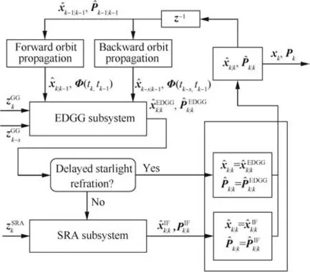
Fig.3 Information fusion filter based on a sequential processing mechanism.

The furthe r state correction from SRA measurements is

with

4.Simulation results and analysis

In this section,the performance ofintegrated navigation using epoch-differenced gravity gradients and starlight refraction is tested with simulated data.Several impact factors such as differencing intervals and orbital heights are also analyzed.

4.1.Simulation conditions

The simulation covers an 18-h data arc starting at 5 December 2015,12:00:00.0(UTC).The truth orbit trajectory is simulated with a high-precision numerical orbit simulator using a 120 × 120 subset of the EGM2008 model for Earth’s nonspherical gravitational attraction,the NRLMSISE-00 model for atmospheric density,the Jet Propulsion Laboratory(JPL)DE405 ephemeris for lunar and solar positions,and the Adams-Bashforth-Moulton method for numerical integration.The LEO satellite under consideration has an orbital height of 300 km.The initial osculating orbital elements are as follows:semi-major axis a=6678.14 km,eccentricity e=0,inclination i=60°,right ascension of ascending node Ω =120°,the argument of perigee ω =0°,and the mean anomaly M=80°.

The truth gravity gradients are generated using a 300×300 subset of the EGM2008 model.The GRF frame is assumed to be always aligned with the satellite Local Vertical Local Horizontal(LVLH)reference frame,where the X-axis is outward along the radial direction(local vertical),Y-axis is perpendicular to X-axis in the orbit plane in the direction of motion(local horizontal),and Z-axis is along the orbit normal.Significant biases having a low drift rate of 0.01 E/h,noise near the orbit frequency with a magnitude of 0.1 E,as well as white noise with a standard deviation of 0.1 E are added to the truth gravity gradients in order to simulate noisy measurements.The precision of both the attitude and refraction star sensors are assumed to be 1 arcsec,with a detectable stellar magnitude of 6.0 and a FOV of 10°× 10°.According to Chen et al.8,at the orbital altitude of 300 km,the GGT observation error caused by an attitude error of 1arcsec is about 0.013 E,which is one order of magnitude lower than the noise level of the simulated gravity gradient measurements.Thus,the effect of attitude error on the EDGG subsystem can be neglected.The installation angle of the refraction star sensor is calculated according to Eq.(14).The Tycho-2 catalogue25is used as the reference catalogue.As stated earlier,the starlight refraction model error is about 0.2 arcsec and is not considered.The measurements are simulated with a data-sampling period of 30 s.

The main filter parameters are set as follows:The initial position and velocity errors are set to[10 km,10 km,10 km,10 m/s,10 m/s,10 m/s]and the diagonal elements of the initial covariance of the state vector are set to[(10 km)2,(10 km)2,(10 km)2,(10 m/s)2,(10 m/s)2,(10 m/s)2].The diagonal elements of the covariance matrix RGGis set to[(0.10 E)2,(0.10 E)2,(0.10 E)2,(0.10 E)2,(0.10 E)2,(0.10 E)2].The standard deviation of the process noise wtis set to 5×10-4m/s2and the standard deviation of ξj，kis set to 1 arcsec.The differencing interval is set to 5.

4.2.Integration performance analysis

Fig.4 Time varying position estimation error for the three orbit determination strategies.

Fig.5 Time varying velocity estimation error for the three orbit determination strategies.

This section compares orbit determination performance between measurements using EDGG only,SRA only,and EDGG+SRA.Time varying position and velocity estimation errors are shown in Figs.4 and 5,respectively,and RMS values of the steady-state estimation error are listed in Table 1.The statistical three-dimensional(3D)error is the root of the sum of the squares of the radial,along-track and cross-track errors.Compared to the orbit determination results presented in Ref.10,the epoch-differencing strategy achieves similar or even better navigation accuracy.The radial and cross-track position errors are especially improved.This indicates the effectiveness of the epoch-differencing strategy in dealing with significant biases and low-frequency noise.Among the three orbit determination methods,the integrated navigation filter converges with the fastest speed and achieves the best accuracy.The 3D Root Mean Square(RMS)position and velocity errors for the integrated navigation are69.175 m and 0.0771 m/s,respectively.Compared to EDGG only orbit determination,the information fusion significantly reduces the along-track position error from 886.41 m to 66.145 m and the radial velocity error from 1.0237 m/s to 0.0735 m/s.It should be noted that the effective accuracy improvements of the se two components are consequences of simultaneous bias and noise reductions.Compared to SRA only orbit determination,the information fusion improves the radial and cross-track position accuracies as well as the along-track and cross-track velocity accuracies.The cross-track position and velocity errors are reduced from 159.58 m and 0.1825 m/s to 15.301 m and 0.0185 m/s,respectively.Overall,the information fusion filter makes the most of both EDGG and SRA measurements and handles the weights of the se two kinds ofobservations properly.As a result,the integrated orbit determination strategy excels over those methods based solely on eithe r gravity gradient or starlight refraction.

Table 1 RMS values of steady-state position and velocity errors for the three orbit determination strategies.

4.3.Influence factors analysis

4.3.1.Effects of differencing intervals

Orbit determination using EDGG+SRA measurements with different differencing intervals(s=1,2,5,10,and 20)is implemented in order to explore the effects of epoch differencing intervals.The RMS values of the steady-state position and velocity estimation errors are summarized in Table 2.It is seen that the orbit determination accuracy improves with the increase of differencing interval.The reason for this lies in the fact that increasing the differencing interval augments the amount of remaining effective information from gravity gradients about the satellite orbit after the differencing operation.As seen in Table 2,the 3D position and velocity errors for s=20 are about half of those for s=1.However,a larger differencing interval requires a longer computation timefor the modeled EDGG measurements.Thus the value of s should be compromised in navigation algorithm design.

4.3.2.Effects of orbital height

The spherical shape of the Earth’s gravitational field indicates that the accuracy of the gravity gradient based orbit determination is highly dependent on orbital height and eccentricity but has little relationship with other orbital elements,such as orbital inclination and argument of perigee.In fact,the eccentricity influences orbit determination accuracy because it causes orbital height to vary with time.In addition,the number of visible refracted stars per orbit period also varies with orbital height.Thus,only the effects of orbital height are analyzed.Asidefrom the 300 km height,another four cases with orbital heights of 600 km,1000 km,1500 km,and 2000 km are also simulated to analyze the effects of orbital height on integrated navigation accuracy.

The RMS values of steady-state position and velocity estimation errors are shown in Table 3.It is seen that the orbit determination accuracy decreases with increasing the orbital height.To be specific,the 3D position error of the 2000 km case is 166.69 m,which is about twice that of the 300 km case.When the orbital height furthe r increases to geosynchronous orbits,the orbit determination error can become unfavorable or unacceptable.This phenomenon can be explained as follows:First,the sensitivity of gravity gradient signals with respect to position decreases with height.The sensitivity factor of GGT has been defined in Ref.8and can be approximately given by 3GM/r4.Second,the number of visible refracted stars is inversely related to orbital height,and the orbit estimation accuracy decreases as the number of visible stars becomes less.The values of GGT sensitivity factors as well as the average number of visible stars per orbit are also given in Table 3.The values of the se two accuracy factors decreasefrom 6.013×10-4E/m and 182 to 2.427×10-4E/m and 88 when the orbital height increases from 300 km to 2000 km.

5.Semi-simulation with real GOCE GGT data

The performance of the integrated navigation filter has also been tested with real GGT data from GOCE combined with simulated SRA measurements.The GOCE is a spaceborne gravity gradiometer launched on 17 March 2009 into a target sun-synchronous near-circular orbit with a height of 278.65 km.A stable and quiet measuring environment is ensured by an electric propulsion engine compensating for non-gravitational forces.Three star sensors and two dualfrequency geodetic GPS receivers are carried to provide highprecision attitude and orbit information.26

An 18-h data arc beginning 8 September 2013,00:00:00.0(GPS Time)is used for the test.The data on this day are reported to be of good quality.The measurements are resampled at intervals of 30 s.Data analysis in Ref.9showed that,in the measurement bandwidth,white noise density levels are on the order of 10 mE/for the,,,andcomponents,whereas for theand Γ）components,the white noise density levels are 350 and 500 mE/respectively.A refraction star sensor onboard GOCE is assumed to provideSRA measurements.The same simulation conditions as those stated in Section 4.1 are used for starlight refraction.

Table 2 RMS values of steady-state position and velocity errors with differencing interval.

Table 3 RMS values of steady-state 3D position and velocity errors as well as accuracy factors with orbital height.

Fig.6 Time varying position estimation error for the GOCE semi-simulation.

Fig.7 Time varying velocity estimation error for the GOCE semi-simulation.

The initial position and velocity errors are set to 10 km and 10 m/s.The standard deviation of the process noise wtis set to 5×10-4m/s2.The diagonal elements of the covariance matrix RGGis setto [(0.01 E)2,(0.01 E)2,(0.01 E)2,(0.35 E)2,(0.01 E)2,(0.50 E)2].The standard deviation of ξj，kis set to 1 arcsec.

The GPS-derived orbits serve as true values for accuracy analysis.The time-varying position and velocity estimation errors are shown in Figs.6 and 7,respectively.The RMS values of steady-state position and velocity errors are summarized in Table 4.Similar to the simulation results,the integrated navigation filter converges the fastest and achieves the best accuracy for the GOCE semi-simulation.The 3D RMS position and velocity errors for the integrated navigation are 98.925 m and 0.1116 m/s,respectively.Compared to EDGG only orbit determination,the integration reduces the along-track position error from 591.34 m to 88.538 m and the radial velocity error from 0.6997 m/s to 0.0961 m/s.Compared to SRA only orbit determination,the integration improves the radial and cross-track position accuracies as well as the along-track and cross-track velocity accuracies.

6.Conclusions

(1)The performance of integrated gravity gradiometry and starlight refraction for LEO autonomous orbit determination has been demonstrated in this study.The integration is implemented by an information fusion filter based on a sequential EKF mechanism,which better addresses asynchronous measurements of multiple sensors.The gravity gradients are time differenced to eliminate slowly varying measurement biases and noise near the orbit revolution frequency.The refraction angle measurements are directly used and its Jacobian matrix derived from an implicit observation equation.This significantly improves the along-track position accuracy compared to thosemethodssolely using gravity gradientsand improves radial and cross-track position accuracies overthose achieved from only using starlight refraction.A three-dimensional position accuracy of better than 100 m is achieved in semi-simulation with real GOCE data.

Table 4 RMS values of steady-state position and velocity errors for the GOCE semi-simulation.

(2)Increasing the differencing interval augments the amount of the remaining effective information for gravity gradients about the satellite orbit after the differencing operation and thus improves the orbit determination accuracy.Orbit determination accuracy decreases with increasing orbital height due to its inverse relationship with the sensitivity of gravity gradient signals as well as the number of visible refracted stars.

(3)The proposed orbit determination method is immune to the signal blockage and spoofing encountered in GPS navigation.Compared to other navigation approaches such as those based on magnetic fields and X-ray pulsars,which typically have position error of several kilometers,much better accuracy,in the tens of meters,has been achieved.

Acknowledgements

This research was supported by the National Natural Science Foundation of China(No.11002008)and has been funded in part by Ministry of Science and Technology of China(No.2014CB845303).The European Space Agency provided the GOCE data.The authors appreciate the valuable remarks of the reviewers and the editors.

1.Nagarajan N,Seetharama Bhta M,Kasturirangan K.A novel autonomous orbit determination system using Earth sensors(scanner).Acta Astronaut 1991;25(2):77–84.

2.Ashkenazi V,Chen W,Hill CJ,Moore T,Stanton D,Fortune D,et al.Real-time autonomous orbit determination of LEO satellites using GPS.Proceedings of the 10th international technical meeting of the satellite division of the institute of navigation;1997.p.755–61.

3.Montenbruck O,Ramos-Bosch P.Precision real-time navigation of LEO satellites using global positioning system measurements.GPS Solut 2008;12(3):187–98.

4.Liu J,Fang JC,Kang ZW,Wu J.Novel algorithm for x-ray pulsar navigation against doppler effects.IEEE Trans Aerosp Electron Syst 2015;51(1):228–41.

5.Hisamoto CS,Sheikh SI.Spacecraft navigation using celestial gamma-ray sources.J Guid Control Dyn 2015;38(9):1765–74.

6.Qian H,Sun L,Cai J,Huang W.A starlight refraction scheme with single star sensor used in autonomous satellite navigation system.Acta Astronaut 2014;96(1):45–52.

7.Farahanifar M,Assadian N.Integrated magnetometer-horizon sensor low Earth orbit determination using UKF.Acta Astronaut 2015;106:13–23.

8.Chen P,Sun X,Han C.Gravity gradient tensor eigendecomposition for spacecraft positioning.J Guid Control Dyn 2015;38(11):2200–6.

9.Sun X,Chen P,Macabiau C,Han C.Low-Earth orbit determination from gravity gradient measurements.Acta Astronaut 2016;123:350–62.

10.Sun X,Chen P,Macabiau C,Han C.Autonomous orbit determination via Kalman filtering of gravity gradients.IEEE Trans Aerosp Electron Syst 2016;52(5):2436–51.

11.O’Hanlon BW,Psiaki ML,Bhatti JA,Shepard DP,Humphreys TE.Real-time GPS spoofing detection via correlation of encrypted signals.Navigation 2013;60(4):267–78.

12.Courtillot V,Le Mouel JL.Time variations of the Earth’s magnetic field:From daily to secular.Ann Rev Earth Planet Sci 1988;16(16):389–476.

13.Moore P,Zhang Q,Alothman A.Annual and semiannual variations of the Earth’s gravitational field from satellite laser ranging and CHAMP.J Geophys Res:Solid Earth 2005;110(B6):B06401.

14.Han K,Wang H,Tu B,Jin Z.Pico-satellite autonomous navigation with magnetometer and sun sensor data.Chin J Aeronaut 2011;24(1):46–54.

15.Wu J,Liu K,Wei J,Han D,Xiang J.Particle filter using a new resampling approach applied to LEO satellite autonomous orbit determination with a magnetometer.Acta Astronaut 2012;81(2):512–22.

16.Wang X,Ma S.A celestial analytic positioning method by stellar horizon atmospheric refraction.Chin J Aeronaut2009;22(3):293–300.

17.Ning X,Wang L,Bai X,Fang J.Autonomous satellite navigation using starlight refraction angle measurements.Adv Space Res 2013;51(9):1761–72.

18.Lillestrand RL,Carroll JE.Horizon-based satellite navigation system.IEEE Trans Aerosp Navig Electron 1963;9(1):127–31.

19.White RL,Thurman SW,Barnes FA.Autonomous satellite navigation using observations of starlight atmospheric refraction.Navigation 1985;32(4):317–33.

20.White RL,Gounley RB.Satellite autonomous navigation with SHAD.Massachusetts:The Charles Stark Draper Laboratory;1987.

21.Wang X,Xie J,Ma S.Starlight atmospheric refraction model for a continuous range of height.J Guid Control Dyn 2010;33(2):634–7.

22.Heiskanen WA,Moritz H.Physical geodesy.San Francisco:W.H.Freeman and Company;1967.

23.Petit G,Luzum B,Al E.IERS conventions(2010).IERS Tech Note 2010;36:1–95.

24.Carlson NA.Federated filter for fault-tolerant integrated navigation systems.Proceedings of IEEE position location and navigation symposium;1988.

25.Høg E,Fabricius C,Makarov VV,Urban S,Corbin T,Wycoff G,et al.The tycho-2 catalogue of the 2.5 million brightest stars.Astron Astrophys 2000;355:27–30.

26.Floberghagen R,Fehringer M,Lamarre D,Muzi D,Frommknecht B,Steiger C,et al.Mission design,operation and exploitation of the gravity field and steady-state ocean circulation explorer.J Geodesy 2011;85(11):749–58.

11 October 2016;revised 10 November 2016;accepted 21 January 2017

Available online 11 July 2017

Autonomous orbit determination;

Epoch-differenced gravity gradients;

GOCE;

Information fusion filter;

Navigation;

Starlight refraction

*Corresponding author.

E-mail address:sunxiucong@gmail.com(X.SUN).

Peer review under responsibility of Editorial Committee of CJA.

Production and hosting by Elsevier

http://dx.doi.org/10.1016/j.cja.2017.07.003

1000-9361©2017 Chinese Society of Aeronautics and Astronautics.Production and hosting by Elsevier Ltd.

This is an open access article under the CC BY-NC-ND license(http://creativecommons.org/licenses/by-nc-nd/4.0/).

©2017 Chinese Society of Aeronautics and Astronautics.Production and hosting by Elsevier Ltd.This is an open access article under theCCBY-NC-NDlicense(http://creativecommons.org/licenses/by-nc-nd/4.0/).