Network Sorting Algorithm of Multi-Frequency Signal with Adaptive SNR

Xinyong Yu, Ying Guo, Kunfeng Zhang, Lei Li and Hongguang Li(.Institute of Information and Navigation, Air Force Engineering University, Xi’an 70077, China; 2.Science and Technology on Information Transmission and Dissemination in Communication Networks Laboratory, Shijiazhuang 05008, China)

Frequency-hopping (FH) communication has been widely used in military communication because of its characteristics of good security, strong anti-interference ability, low probability of interception and strong networking capability. Determining a technique to realize the correct network sorting for multiple frequency hopping signals with different frequency hopping parameters without prior knowledge, is the core problem of frequency hopping signal reconnaissance and countermeasure[1-2].

For the multiple frequency hopping signals network sorting, the traditional algorithm mainly considers the characteristic parameters of FH signals, such as the hop time, amplitude, direction of arrival and so on, but the accuracy is low and the complexity is high[3-7]. The blind source separation method is proposed in Refs. [8-10] to realize the signal sorting of broadband frequency hopping signal. The idea is novel, but this method is only applicable to the orthogonal frequency hopping signal, which is powerless to the frequency hopping signal of asynchronous network. Two independent component analysis methods are proposed in Refs. [11-12] to separate FH signals. But the performance of the algorithm is poor under the condition of low signal noise ratio (SNR) or signal power disparity, and it is only applicable to the over-determined condition. Yang proposed a maximum SNR blind source separation method in Ref.[13]. For asynchronous non-orthogonal FH signals, the separation accuracy is high and fast, but for synchronous orthogonal FH signals, the accuracy is greatly reduced. The algorithm lacks universal applicability. Then Sha proposed an improved subspace projection method to realize the network separation under undetermined conditions, but the SNR adaptive capacity is weak, where the minimum SNR is 10 dB.

Based on the above issues, aiming at the multi-FH signal sorting under undetermined and low SNR condition, in accordance with the “two step” method, this paper put forward a SNR-adaptive sorting algorithm using the time-frequency (TF) sparsity of FH signal. The hybrid frequency hopping signal is transformed by the Gabor transform, and the model of network sorting is constructed. Secondly, the mixing matrix is estimated accurately by the TF ratio matrix of TF single source point, and then an improved subspace projection method is used for network sorting. In order to improve the performance of network sorting under low SNR condition, the adaptive SNR TF pivot threshold method is used to find the TF single source point, and the AP clustering method is used to cluster the column vectors of TF ratio matrix. Finally, the algorithm in Ref. [14] is used as the reference algorithm and the simulation results using the two algorithms are compared as well.

1 Mathematical Model

1.1 FH signal model

Suppose that the hopping period of FH signal sn(t) isT, there areKhops within time of Δtin total.ωnkandφnkrepresent the carrier frequency and initial phase ofK-th hop respectively and the time of initial hop is Δt0n. Then sn(t) can be written as[15]

(1)

wheret′=t-(k-1)Tn-Δt0n,υnstands for the complex envelope of base band of signal sn(t), andrectis the unit rectangle pulse.

Suppose thatNFH signals s(t)=[s0(t) …sN-1(t)]Timpinge instantaneously onto anM-element array and the elements in the array are isotropic. Regardless of the effects of channel inconsistency and mutual coupling, the system model can be formulated as

x(t)=As(t)+v(t)

(2)

where x(t)=[x0(t) …xM-1(t)]Tis observation signal; A=[a0…aN-1]T⊂CM×Nis anm×ncomplex valued mixing matrix whose columns are full rank; and v(t)=[v0(t),…,vM-1(t)]Tis the white Gaussian noise signal with zero mean value and varianceδ2, and the signal is not correlated with it.

In this paper, multi-FH signal sorting under undetermined condition refers to the situation that the number of FH signal is greater than the received elements i.e.N>M. Since the mixing matrix A is unknown, we need to estimate the mixing matrix firstly. Since Eq.(2) has infinite solutions, we need to use the method of blind separation to solve it.

1.2 Multi-FH signal sorting model

TF domain is chosen as the sparse domain because of the good sparsity of FH signal domain. Since the TF ratio matrix is used in the estimation of the mixing matrix, the TF transformation of the observation signal should be linear. The short-time Fourier transform (STFT) and the Gabor transform are both commonly used linear transformations. The Gabor transform is the optimal linear transform whose window is a Gaussian window, which is the function when the window of time domain reaches its minimum. The localization of TF can be achieved as long as the area reaches the lower bound of the uncertainty principle. So the Gabor transform is chosen as the TF transform of the system.

Since the Gabor transform is a linear TF distribution, we can rewrite the model from Eq.(2) as

X(t,f)=AS(t,f)+V(t,f)

(3)

where X(t,f)=[X0(t,f) …XM-1(t,f)]T, S(t,f)=[S0(t,f) …SN-1(t,f)]Tand V(t,f)=[V0(t,f) …VM-1(t)]Tare the Gabor transform of observation signal x(t), source signal s(t), and additive noise signal v(t) respectively. Eq. (3) represents the model of multi-FH signal sorting under undetermined condition in the TF domain.

2 Estimation of the Mixing Matrix

2.1 Adaptive SNR pivot threshold setting

(4)

whereεis a threshold of TF pivot point. It can be seen that if the thresholdεis too small, the corresponding TF points of noise will be misinterpreted as TF pivot points. On the other hand, if the thresholdεis too large, some TF support points will be filtered out. In Ref. [14], although the effect of noise is considered, the threshold is set as three times of the noise variance, i.e.ε=3σn, (σnis the noise variance). As a result, the threshold is set too low to filter the noise out which directly influences the effect of subsequent network sorting. In order to solve this problem, the SNR adaptive pivot threshold setting method is proposed. This method takes all the TF points in TF domain into consideration and uses an iterative algorithm to calculate the threshold value. Since the value of TF points varies with the SNR, the threshold has adaptive SNR characteristics.

The main idea of the algorithm is to find the minimum and maximum frequency module valueW1andWkof all TF points and the initial thresholdε1firstly

ε1=(W1+Wk)/2

(5)

Then divide the TF points into two parts TF1, TF2withε1as the TF pivot point threshold. Calculate the number of TF points and average frequency module values of the two regions as

(6)

whereWtfis the frequency module value ofx(t,f). A new threshold is calculated according to the average frequency module value of the two regions.

εK=(Wtf1+Wtf2)/2

(7)

Finally, the threshold is updated using the iterative idea according to the above method. The final iteration is determined until the (K+1)-th result equals theK-th result (i.e.εK+1=εK).

2.2 Mixing matrix estimation based on the TF ratio matrix

X(t,f)=akSk(t,f)+V(t,f)

(8)

Despite the influence of noise, the TF ratio matrix of observation signals of each receiving array to them-th receiving array is expressed as

(9)

It is visible that all columns of the ratio matrix in Eq.(9) are identical, so if we obtain the TF single-source point set the mixed matrix A can be estimated by

(10)

Considering the noise, the columns of the ratio matrix in Eq.(9) are different from each other, but have significant clustering characteristics.

The mixing matrix estimation algorithm is summarized as follows.

Step1Calculate the Gabor transform of the mixed signals X(t,f) to get the network sorting model by Eq.(3).

Step2Calculate the initial thresholdε1according to the TF point of mixed signals in TF domain by Eq.(5).

Step3Calculate the average frequency module value of the two regions by Eq.(6), and get the new thresholdεKby Eq.(7).

Step4Start threshold iteration, ifεK+1=εK, then stop the iteration to get the final thresholdεK, otherwise go to step 2.

Step5Get all the TF pivot points by Eq. (4).

Step6Get the TF ratio matrix W of TF pivoting domain by Eq.(9).

Step7Calculate the similarity matrix S of column vector data of W, attraction degree and attribution degree.

Step8Determine the cluster center according to the judging condition, and get the TF single source setΛ(1),…,Λ(N).

Step9Calculate the estimated mixed matrix by Eq.(10).

3 Network Sorting under Undetermined Condition

The improved subspace-based algorithm is used to sort the network, when the number of true FH signal sources is less than the hypothetical sources. Considering the influence of noise, there are not only noise residuals, but also the FH source signal residuals at the time point when calculating the orthogonal projection of the mixed matrix. So the general subspace-based algorithm will lead to non-ideal sorting effect. To solve this problem, Sha[14]proposed an improved subspace-based algorithm for undetermined network sorting to relax sparsity constraints. The improved subspace-based algorithm introduces the comparative powers of sources to the conventional subspace-based algorithm. The comparative powers of the source is set as an index of the FH network sorting. By combining the mixing matrix and comparative powers, the new algorithm can deal with the case whereK≤Mat any TF point. The relative power of the FH signal source can be defined as

(11)

where ‖·‖2denotes the 2-norm andLkdenotes the number of vectors contained in the setΛnof time-frequency source.

Suppose that the number of sources in each TF point isR, and the mixing matrix column vector of the corresponding FH source signal at the TF point (t′,f′) is AR=[an1…anR], so the FH signal network sorting model at the TF point can be expressed as

X(t′,f′)=ARSR(t′,f′)+V(t′,f′)

(12)

where SR(t′,f′)=[Sn1(t′,f′),…,SnR(t′,f′)]. Let H presents the orthogonal project matrix onto noise subspace of ARwhen the number of source signals at TF point (t′,f′) is less than the number of receiving elements. H is expressed as

(13)

where I denotes the unit matrix. Taking the noise into account, ARis estimated as

(14)

The source signal S(t′,f′) can be calculated by Eq. (12) and Eq. (14) in the case of known ARso as to realize the network sorting. When the number of source signals on the TF point (t′,f′) is equal to the number of receiving array elements, a thresholdεassociated with the relative power deviation of the source signal is used to determine in which case the number of source signal is equal to the number of receiving array elements.

SinceR=M′, we can rewrite the model from Eq.(12) as

X(t′,f)=an1Sn1(t′,f′)+…+
anMSnM+V(t′,f′)

(15)

Eq.(15) can be expressed in the form of relative power as

X(t′,f′)=an1En1ejθn1+…+
anMEnMejθnM+V(t′,f′)

(16)

whereaniEniejθnidenotes the relative power of the FH source signal Sni(t′,f′). The TF active sources at TF point (t′,f′)are estimated by

(t′,f′)=A-1X(t′,f′)

(17)

The network sorting algorithm is summarized as follows.

Step1Calculate the FH signal network sorting model at the TF point by Eq.(12).

Step2LetR=M-1, calculate the orthogonal project matrix by Eq.(13).

4 Simulation and Analysis

Suppose that the number of received array elementsM=2, the spacing of the elements is 2.5 m, the receiver processing bandwidth is[20 MHz, 500 MHz], and the sampling frequency is 1 000 MHz. In order to meet the narrow-band assumption, the FH signal frequency is set asfRF=10 GHz. The signal parameters of five sources are summarized in Tab.1.

Tab.1 Parameters of FH source

4.1 TF distribution of observation signal

Fig. 1 is the TF distribution of proposed algorithm and reference algorithm in the situations that source signals are S0,S1,S2respectively while SNR=5 dB. It can be seen from Fig. 1 that under the same SNR, the TF spectrum of the proposed algorithm has strong focusing capability and small noise interference which lays a good foundation for the subsequent TF ratio matrix calculation.

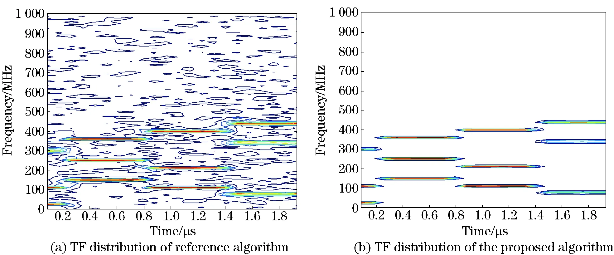
Fig.1 Comparison between T-F images of observed signal

4.2 Multi-FH signal network sorting

Fig. 2 is the TF distribution of network sorting results of the source signals S0,S1,S2,S3at SNR=0 dB in the proposed algorithm and reference algorithm. It can be seen from Fig. 2 that compared with the reference algorithm the TF distribution of the FH source signal of proposed algorithm is not affected by the noise and cross-interference term, and the energy of signal spectrum is more concentrated. The proposed algorithm can obtain four FH networks from the mixed signals of the received array elements effectively.

Fig.2 FH sorting result comparison

In order to measure the performance of multi-FH signal network sorting, the signal-to-interference ratio (SIR) is taken as the criterion. The SIR is defined as

(18)

Fig. 3 displays how the SIR of the proposed algorithm and the reference algorithm changes with the increase of SNR from 0 dB to 35 dB using Monte-Carlo simulation, when the source signals are S0,S1,S2,S0,S1,S2,S3,S0,S1,S2,S3,S4and the array elements remain the same. The results show that our algorithm reaches its limit when SIR=10 dB while the reference algorithm reaches its limit when SIR=15 dB. The sorting performance of the reference algorithm processing source signalN=3 is better thanN=4, but when the number of frequency hopping source signals reaches 5, the sorting performance is greatly reduced, regardless of the SNR; The sorting performance of the proposed algorithm is almost the same whenN=3, 4, 5, and the SIR does not decrease with the increase of FH signal.

Fig.3 Comparison of SIR

5 Conclusion

Under the environment of intensified electronic warfare, especially in wartime, frequency-hopping network density is high, and it is easy to encounter under-determined condition. Multi-FH signal network sorting under undetermined condition is of great significance. We have introduced undetermined blind separation algorithm based on sparse representation to sort the FH signals. The adaptive-SNR threshold setting method improves estimation performance under low SNR conditions. Simulations demonstrated that the new algorithm can separate the FH signals efficiently in low SNR conditions.

[1] Fu Weihong, Wang Lu, Jia Kun, et al. Blind parameter estimation algorithm for frequency hopping signals based on STFT and SPWVD[J]. Journal of Huazhong University of Science and Technology, 2014(42): 59-63. (in Chinese)

[2] Sha Z C, Liu Z M, Huang Z T. Online hop timing detection and frequency estimation of multiple FH signals[J]. Etri Journal, 2013,35(5): 748-757.

[3] Zhang Dongwei, Guo Ying, Qi Zisen, et al. Joint estimation algorithm of direction of arrival and polarization for multiple frequency-hopping signals[J]. Journal of Electronics & Information Technology, 2015,37(7): 1695-1701. (in Chinese)

[4] Zhang Dongwei, Guo Ying, Qi Zisen, et al. A joint estimation algorithm of multiple parameters for frequency hopping signals using spatial polarimetric time frequency distributions[J]. Journal of Xi’an Jiaotong University, 2015,49(8):17-23. (in Chinese)

[5] Lin C H, Fang W H. Joint angle and delay estimation in frequency hopping system[J]. IEEE Transactions on Aerospace and Electronic Systems， 2013,49(2):1042-1056.

[6] Fu W H, Hei Y Q, Li X H. UBSS and blind parameters estimation algorithms for synchronous orthogonal FH signals[J]. Journal of System Engineering and Electronics, 2014,25(6)： 911-920.

[7] Liu X Q, Nicholas D S, Swami A. Joint hop timing and frequency estimation for collision resolution in FH networks[J]. IEEE Transactions on Wireless Communications， 2005,4(6): 3063-3074.

[8] Wong K T. Blind beamforming/geolocation for wideband-FFHs with unknown hop-sequences[J]. IEEE Transactions on Aerospace and Electronic Systems, 2001,37(1): 65-76.

[9] Zhang Chaoyang, Cao Qianqian, Chen Wenzheng. Blind separation parameter estimation of multiple frequency-hopping signals[J]. Journal of Zhejiang University, 2005,39(4)： 465-470. (in Chinese)

[10] Comon P, Jutten C. Handbook of blind source separation: independent component analysis and application[M]. New York: Academic Press,2010.

[11] Chen Chao, Gao Xianjun, Li Dexin. Overlapped frequency-hopping communication signals separation algorithm based on independent component analysis[J]. Journal of Jilin University, 2008,26(4): 347-353. (in Chinese)

[12] Cardoso J F, Donoho D I. Equivariant adaptive source separation[J]. IEEE Trans Signal Processing, 1996,44(12): 3017-3030.

[13] Yang Baoping, Chen Yongguang, Yang Luan, et al. A blind separating method for asynchronous nonorthogonal frequency hopping network[J]. High Power Laser and Particle Beams, 2015,27(10): 103251-1-103251-6. (in Chinese)

[14] Sha S C, Huang Z T, Zhou Y Y, et al. Frequency-hopping signals sorting based on underdetermined blind source separation[J]. IET Communications, 2013,7(14): 1456-1464.

[15] Fu K C, Chen Y F. Blind iterative maximum likelihood-based frequency and transition for frequency hopping systems[J]. IET Communications, 2013,7(9):883-892.