Numerical simulation of wind-driven circulation and pollutant transport in Taihu Lake based on a quadtree grid

Xiao-dong Liu , Ling-qi Li , Peng Wang , Zu-lin Hua ,*, Li Gu ,Yuan-yuan Zhou , Lu-ying Chen

a Key Laboratory of Integrated Regulation and Resource Development on Shallow Lakes of Ministry of Education, Nanjing 210098, China

b College of Environment, Hohai University, Nanjing 210098, China

Abstract In this study,a two-dimensional flow-pollutant coupled model was developed based on a quadtree grid.This model was established to allow the accurate simulation of wind-driven flow in a large-scale shallow lake with irregular natural boundaries when focusing on important smallscale localized flow features. The quadtree grid was created by domain decomposition. The governing equations were solved using the finite volume method, and the normal fluxes of mass, momentum, and pollutants across the interface between cells were computed by means of a Godunov-type Osher scheme.The model was employed to simulate wind-driven flow in a circular basin with non-uniform depth.The computed values were in agreement with analytical data. The results indicate that the quadtree grid has fine local resolution and high efficiency, and is convenient for local refinement. It is clear that the quadtree grid model is effective when applied to complex flow domains. Finally, the model was used to calculate the flow field and concentration field of Taihu Lake,demonstrating its ability to predict the flow and concentration fields in an actual water area with complex geometry.

Keywords: Numerical simulation; Wind-driven circulation; Pollutant transport; Quadtree grid; Shallow-flow hydrodynamics; Taihu Lake

1. Introduction

The hydrodynamics of shallow lakes,coastal lagoons,wide rivers, and estuaries can be simulated using depth-averaged shallow water equations (SWEs). In current research, the hydrodynamic model is based on two-dimensional (2D) SWEs,while an advection-diffusion equation is used for simulation of pollutant transport. The issue of dispersion needs to be considered when using shallow-water dynamics for pollutant transport research. For environmental flow, numerical models based on nonlinear SWEs may be suitable for adequately describing significant hydraulic processes. In some cases, regions with rapid changes in flow and local areas that are relatively important are included in a domain, which may require local grid refinement. Various approaches have been proposed for adaptive grid resolution to improve the computational efficiency of SWEs (Sleigh et al., 1998; Liang et al.,2004, 2007; Skoula et al., 2006). Typical grid generation techniques can be classified as either structured or unstructured grids, each of which has specific advantages and disadvantages (Dadone and Grossman, 2007; Tavakoli, 2008). In particular, the rectangular grid has a simple data structure,high processing efficiency,and adequate orthogonality,as well as other features, which allow it to be used widely in flow simulation. However, when using the rectangular grid to fit natural waters,the boundaries will be fitted poorly if the grid is very coarse. Bennett and Clites (1987) demonstrated that the presence of coarse cells at the boundaries can lead to the erroneous prediction of particle paths, whereas excessively fine cells will increase the computational load. Thus, it is difficult to simulate flow in water areas with complex natural boundaries and to refine local cells. Significant efforts have been made to develop advanced adaptive grid technologies,and the quadtree hierarchical grid,proposed in recent years,is an effective method for treating complex boundaries.

The quadtree grid technique was first proposed by Yerry and Shephard (1983), with its first applications in computer graphics, image processing, and geographic information systems(Samet,1990).Its first application to computational fluid dynamics was in the aerospace field (DeZeeuw and Powell,1993). The quadtree grid is created by recursive subdivision of seeding points. Research into the application of quadtree grids to hydrodynamics was originally based on a fixed grid(G′asp′ar et al.,1994;Rogers et al.,2001),but the disadvantage of this method is that the resolution is inadequate throughout the flow domain when the method is applied to cases with complex boundaries, or cases in which the hydrodynamic features change rapidly over small distances. In order to overcome these problems,Borthwick et al.(2001)and An and Yu (2014) employed adaptive quadtree grid models that can approximate any 2D boundaries and are easier to refine or coarsen. The quadtree technique has also been used to simulate nonlinear waves (Greaves et al., 1997), separated flows(Greaves and Borthwick, 1998), wave-current interactions(Zhang et al., 2012), and wave runups (Cho et al., 2004).Water pollution has long been recognized to be of major importance to public health.Recently,some research has been conducted to apply quadtree grids to the simulation of pollutant transport (Copeland et al., 2003; Hua et al., 2003).

In this study,we used a quadtree grid shallow flow-pollutant coupled model to simulate wind-driven circulation and pollutant transport. The numerical model was validated using a standard benchmark test on the wind-driven flow in a circular domain.Then,the model was used to simulate the real case of the winddriven circulation and pollutant transport in Taihu Lake.

2. Quadtree grid generation

2.1. Grid generation

The quadtree grid generation method employed in this study was based on the principle described here. The first step in generating a satisfactory quadtree grid is to define a set of seeding points that adequately describe the domain boundaries and any internal areas of interest (e.g., areas with large gradients).The physical flow domain is rescaled so that it fits into an initial square cell,and the maximum and minimum sizes for the cells are specified.A primary quadtree grid is then generated by recursively subdividing the initial square cell according to the criterion that a cell is subdivided when it contains two or more seeding points or the size of subdivided cells is greater than the maximum size. The quadtree grid is then regularized to ensure that no cell has a side length of more than twice that of its neighbors,thereby restricting the number of hanging nodes.The steps for quadtree generation are summarized in Fig. 1. A complete description is provided by Liang et al. (2004).

2.2. Elevation interpolations

The elevation of each cell needs to be determined to perform further simulation. Elevation interpolation is used to determine the value of each cell. Various interpolation methods have been proposed, such as nearest neighbor interpolation (Surhone et al., 2013), inverse distance weighted(IDW) interpolation (Lima et al., 2003), thin plate spline interpolation (Tait et al., 2006), and triangle interpolation(Jiang, 2014). In this study, we used the triangle interpolation method to obtain the bottom elevation. Fig. 2 illustrates the procedure for triangle interpolation based on the digital elevation model(DEM),where P1,P2,and P3are the nodes of a triangular element, and O1through O4are the points whose elevations are obtained through linear interpolation.

3. Numerical model

3.1. Governing equations

The 2D nonlinear shallow water and pollutant transport equations may be derived by depth-integrating the threedimensional Reynolds averaged Navier-Stokes equations. A conservation law for the equations may be written in the matrix form as

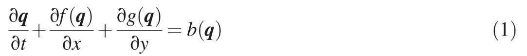
Fig. 1. Steps for generation of quadtree grid.

where q=（h,hu,hv,hC）Tis a conserved physical vector,with h being the water depth, C being the pollutant concentration, and u and v being the velocity components in the x- and y-directions, respectively; t is time; f（q）=（hu,hu2+gh2/2,huv,huC）Tis the flux vector in the xdirection,with g being the gravitational acceleration;g（q）=（hv,huv,hv2+gh2/2,hvC）Tis the flux vector in the ydirection; and b（q）=（b1,b2,b3,b4）Tis a source/sink term,with b1= 0, b2= gh（S0x- Sfx）, b3= bh（S0y- Sfy）, and b4= ∇·[Di∇（hC）]+ S/A- KhC, where S0xand Sfxare the bed slope and friction slope in the x-direction, respectively,S0yand Sfyare the bed slope and friction slope in the y-direction, respectively, b is the width of the water area, Diis the horizontal diffusion coefficient, K is the degradation coefficient, S is the source/sink term for each pollutant, and A is the area of a cell.

Fig. 2. Steps for interpolation.

3.2. Finite volume method

After integrating Eq. (1) over an arbitrary cell, the basic equation for the finite volume method (FVM) obtained using the divergence theorem is given by

where dω and dL are areal and arc elements of the domain with an area of Ω, respectively, n is a unit outward vector normal to the boundary Γ,and F（q） =（f（q）,g（q））T.Based on first-order accuracy discretization and the rotation invariance property of f（q）and g（q）on each side of the cell(Hemker and Spekreijse,1985),the following equation can be derived from Eq. (2):

whereφistheanglebetweenthevectornandthex-axis(measured counterclockwise from the x-axis);is the transformed form of q,= T（φ）q; T（φ） and T（φ）-1are the transformation and inverse transformation matrices, respectively; m is the total number of sides of a cell;Ljis the length of side j;and b*（q） =（Ab1,Ab2,Ab3,∑Di[∇（hC）]nLj+S-AKhC）,where[∇（hC）]nmeans the component of ∇（hC） in the normal direction.The q states on the left and right sides of the interface are different,and the outward normal flux Fandis calculated by solving the initial Riemann problem.Then,a Godunov-type Osher scheme(Zhao etal.,1994)isusedtocalculatethenumericalfluxontheboundary.

4. Results and discussion

4.1. Numerical simulation of wind-driven circulation in a circular basin

To check the produced 2D quadtree grid model, we performed a numerical test of wind-driven circulation in a nonuniform-depth circular basin. Simulations were performed using a quadtree grid and a rectangular grid.

In the test, uniform wind stress was applied to the shallow water surface of a circular dish-shaped basin with a radius of 193.2 m and non-uniformly varying bathymetry (Fig. 3). The depth-averaged velocities in deeper water were directed against the wind stress, whereas in shallower water, the velocities were more likely to be in the same direction as the applied wind stress.In this case,the wind speed U was 4 m/s,from the southeast. There was no Coriolis force in this case.

Fig. 4 illustrates the computational grid at a maximum resolution level of 8, which corresponds to the boundary of the refined quadtree grid with Δx = Δy = 2.5 m. The resolution level of the grid at the exterior of the simulation domain is 4,which corresponds to Δx = Δy = 40 m. At the center of the basin, the resolution level is 6, which corresponds to Δx =Δy = 10 m. There are 3304 grid cells in total.

Fig. 3. Bathymetry of circular dish-shaped basin (units: m).

To confirm the convergence of the quadtree grid, flow patterns were simulated on a uniform grid and a quadtree grid,with the time step in the simulation set at Δt = 1 s. Fig. 5(a)depicts the depth-averaged velocity distribution at a steady state in the basin, which was obtained using the uniform grid with a resolution level of 6. Fig. 5(b) shows the depthaveraged velocity distribution at a steady state obtained with a quadtree grid, which confirms the position of the gyres within the basin. We found that the velocity distributions obtained with the two grids are very similar, except at the position immediately adjacent to the boundaries where the effects of the gradient approximation are evident on the quadtree grid. The flow pattern is diametrically symmetric with respect to the wind direction.Two counter-rotating gyres can be seen,and the flow across the deepest part of the basin is directed against the wind direction.The centers of the gyres lie slightly downwind of the north-south center line of the basin,thereby agreeing with the results obtained by Roger et al.(2001) and Borthwick et al. (2001).

The models were also compared by plotting the normalized depth-averaged velocity (Rogers et al., 2001). Kranenburg(1992) assumed a stable flow, and the analytical solution was calculated as follows:

Fig. 4. Quadtree grid for circular basin.

Fig. 5. Computed wind-driven velocity fields in circular dish-shaped basin.

where U is the depth-averaged velocity; u*is the surface friction velocity, andwith τwbeing the wind shear stress, and ρ being the density of water; κ is the Karman constant, and κ = 0.4; Z = H/z0, where H is the weighted mean water depth, and z0is the bottom roughness,with z0= 0.0028 m; r is the distance from the center of the basin; and R is the radius of the basin.

A comparison of a simulated profile and Kranenburg's theoretical prediction is shown in Fig.6,with the axis of radial location directed from southwest to northeast. It demonstrates that there is an agreement in the general behavior of the normalized depth-averaged velocity, although the numerical results do not include a kink at the center of the basin,and they are also more oscillatory than the analytical profile.According to Fig. 6, the coefficient of correlation between quadtree grid calculations and analytical values is 0.982, and the root mean square error (RMSE) is 0.0432. However, the coefficient of correlation between rectangular grid calculations and analytical values is 0.925,with the value of RMSE being 0.124.The calculated results of the quadtree grid model are closer to the analytical values, compared with those obtained with the uniform grid without local encryption. In particular, for the region near the boundary where the quadtree grid is encrypted,the precision of the calculated results is higher than that of the uniform grid without local encryption. Overall, this test validates the efficacy of the new quadtree model in solving SWEs using Roe's approximate Riemann solver.

4.2.Numerical simulation of wind-driven circulation and pollutant transport in Taihu Lake

Fig. 6. Comparison of normalized depth-averaged flow velocity profiles in circular dish-shaped basin.

The model was also employed to simulate wind-driven circulation and concentration fields in Taihu Lake, the third largest freshwater lake in China. It is located 100 km west of Shanghai. The lake has an area of approximately 2445 km2and an average depth of 1.89 m. Its bathymetry is shown in Fig. 7. The lake is a major tourist attraction as well as a drinking water source for Wuxi, Shanghai, and other cities in Eastern China. However, due to the rapid growth of industry and the population in the lake basin, large quantities of industrial waste, sewage, and agricultural wastewater have been discharged into the lake, but the wastewater treatment facilities in these areas are inadequate. Water pollution caused by industrial and agricultural effluents has resulted in poor water quality and severe eutrophication in Taihu Lake. In particular,a blue algal bloom in Taihu Lake worsened its water quality and severely affected the drinking water supply for two million residents of Wuxi City in 2007.

For aid in analysis of the characteristics of the winddriven circulation in Taihu Lake, Fig. 8 shows a threelevel quadtree grid for the lake, which was generated around perimeter seeding points. The grid contains 9851 interior cells and 10306 nodes. The computational region was divided into three parts, with cells of different scales.The cells were refined in the locally important regions(Zhushan Lake and Meiliang Lake) and at the boundary,

Fig. 7. Bathymetry of Taihu Lake.

where Δx = Δy = 250 m. In the western part of the lake,the dimensions of cells are Δx = Δy = 500 m, while in the other regions, Δx = Δy = 1000 m. Fig. 9(a) shows the wind-driven circulation predicted using the quadtree grid model, subject to southeasterly wind with a speed of 3.5 m/s and an assumed wind drag coefficient of 0.0013. The calculated circulation structure is consistent with the observed flow field structure (Fig. 9(b)), and thus it can reflect the characteristics of the wind-driven circulation in Taihu Lake. The flow field is smooth at the intersection between cells with different scales.

To verify the performance of the model, two uniform grids were used to simulate the wind-driven circulation in Taihu Lake.One was a coarse uniform grid with Δx=Δy=1000 m.The other was a fine uniform grid with Δx = Δy = 250 m.Fig. 10 shows the local steady-state velocity distributions for Zhushan Lake subject to southeasterly wind, which were predicted using the quadtree grid model and two uniform grid models. These results show that a pair of steady gyres can be found in the flow field obtained using the quadtree grid. However, the gyres are not clearly shown in Fig. 10(b) because the grid is coarse.The flow fields in Fig.10(a)and(c)are smoother than that obtained with a coarser grid in Fig. 10(b). The flow patterns obtained using the quadtree grid model agree with the numerical results obtained using the fine uniform grid model.However, the quadtree grid model was only comprised of 9851 cells,far fewer than those in the fine uniform grid model.Table 1 compares the efficiency of the three models, demonstrating that the quadtree grid is cost-effective, and it handles the wind-driven circulation in an efficient manner.

The effluent source in the model calculation was located at the mouth of the Taigeyun River within the study area. The Taigeyun River is the largest river flowing into Zhushan Lake and its stream discharge rate is 32.38 m3/s. The pollutant distribution near the estuary is influenced by the wind-driven circulation and the nearby runoff. The emission of the chemical oxygen demand(COD)is 32500 t/year.Fig.11 shows the COD concentration contours in Zhushan Lake under the actions of the southeasterly and northwesterly winds,respectively.

5. Conclusions

In this study, we used a 2D numerical model based on a quadtree grid to simulate the wind-driven circulation and pollution dispersion in shallow water. The grid was generated automatically based on seeding points. The elevation of each cell was obtained using triangle interpolation based on the digital elevation model. The governing equations for shallow water flow were solved using the FVM,and the normal fluxes of mass, momentum, and pollutants across the interface between cells were computed by means of a Godunov-type Osher scheme.

The model was used to simulate wind-driven circulation in a circular basin with non-uniform depth. The computed values were in agreement with the analytical data. These results indicate that quadtree grid cells have fine local resolution and high efficiency, and are convenient for local refinement. It is clear that the quadtree grid model is efficient when applied to complex flow domains. Finally, the model was used to simulate the flow field and concentration field in Taihu Lake, demonstrating the applicability of the model to an actual water area with complex geometry.Comparison of the numerical results obtained using different grids shows that the quadtree grid is efficient in controlling the total number of grid cells, while still providing fine resolution at the boundaries and in locally important regions.

Table 1Comparison of efficiency of different grids.

Fig. 11. COD concentration contours in Zhushan Lake subject to winds of different directions (units: mg/L).