
Submerged flexible vegetation impact on open channel flow velocity distribution: An analytical modelling study on drag and friction
2019-07-24 07:35JnPuAwesrHussinkunGuoNikolosVrdkstnisPrshnthHnmihgriDennisLm
Water Science and Engineering 2019年2期
Jn H. Pu *, Awesr Hussin Y-kun Guo Nikolos Vrdkstnis Prshnth R. Hnmihgri , Dennis Lm
a Faculty of Engineering and Informatics, University of Bradford, Bradford BD7 1DP, UK
b Department of Civil Engineering, Indian Institute of Technology, Kharagpur 721302, India
Abstract In this paper, an analytical model that represents the streamwise velocity distribution for open channel flow with submerged flexible vegetation is studied.In the present vegetated flow modelling,the whole flow field has been separated into two layers vertically:a vegetated layer and a non-vegetated free-water layer.Within the vegetated layer,an analysis of the mechanisms affecting water flow through flexible vegetation has been conducted. In the non-vegetated layer, a modified log-law equation that represents the velocity profile varying with vegetation height has been investigated.Based on the studied analytical model,a sensitivity analysis has been conducted to assess the influences of the drag(CD)and friction (Cf) coefficients on the flow velocity. The investigated ranges of CD and Cf have also been compared to published values. The findings suggest that the CD and Cf values are non-constant at different depths and vegetation densities, unlike the constant values commonly suggested in literature. This phenomenon is particularly clear for flows with flexible vegetation, which is characterised by large deflection.
Keywords: Analytical model; Flexible vegetation; Flow velocity; Friction; Drag; Submerged vegetation
1. Introduction
Vegetation is an important design factor for open channel flow.It affects local water depth and velocity profile,and has a varying impact depending on the vegetation type (Han et al.,2016). It is well-accepted that vegetation can hinder flow by acting as an obstruction, generating turbulence, and affecting the entire flow velocity distribution and local water depth, as well as sediment transport (Pu et al., 2014a, 2014b; Pu and Lim, 2014; Pu, 2015). Recent studies have examined the characteristics of flexible aquatic vegetation,which have been found to be significantly different from those of rigid vegetation (Dijkstra and Uittenbogaard, 2010). Velocity profiles within a flow section usually vary with vegetation type and distribution pattern in the open channel. More specifically,velocity distribution can be directly influenced by the vegetation drag due to its high roughness contribution to flow(Wu et al., 1999).
In a vegetated flow, the drag coefficient decreases with the flow Reynolds number (Kothyari et al., 2009). Tanino and Nepf (2008) further stated that the normalised drag force,i.e., the ratio of the mean drag to the product of viscosity and pore velocity, has a linear dependence on the Reynolds number. Ishikawa et al. (2000) reported that the change in drag coefficient varies with the diameter of the vegetation stem;however, its reliance on the Reynolds number was not specified. Cheng and Nguyen (2011) concluded that the hydraulic radius can be used as a more reasonable length scale to describe the flow domain induced by vegetation stems, which yielded a redefined Reynolds number to formulate an improved drag coefficient relationship.
From the studies above, the reaction forces by the vegetation are related to a few key parameters, such as the drag coefficient CDand friction coefficient Cf, which depend on complex factors, such as the vegetation size, Reynolds number, bed slope, and vegetation thickness/dimensions. Thus,assuming a constant value of CDor Cffor different flow and vegetation conditions,as adopted by various researchers,such as Huai et al. (2013), Kubrak et al. (2008), Yang and Choi(2010), and Tsujimoto and Kitamura (1990), may lead to imprecise representation of the flow velocity profile. In order to investigate how CDand Cfchange with flow and vegetation conditions, this study investigated the published experimental data using different CDand Cfvalues to quantify their limits for the investigated vegetated flows.
2. Previous considerations
2.1. Vegetation resistance
Hu et al. (2013) proposed an analytical model to calculate the streamwise velocity across the flow depth,which included vegetation with small bending. Their hypothesis for the calculation of the bending moment of the vegetation stem was that the force exerted on a stem was uniformly distributed.This assumption may not be ideal for flow with fully flexible vegetation.In natural vegetated channels,the determination of an accurate vegetation drag force in flow is complex due to the following factors: (1) most natural vegetation does not resemble a perfect cylinder shape; (2) natural vegetation usually has a higher CDdue to existence of leaves and substems (Jarvela, 2004); (3) highly flexible natural vegetation can flex under flow to adopt a more streamline shape,causing a lower CD(Kouwen and Fathi-Moghadam, 2000); (4) vegetation elements in a population can be sheltered by others to give different drag coefficients compared to an individual element (Nepf and Vivoni, 1999); and (5) free-end drag of submerged vegetation can cause fluctuating disturbance to flow and hence its velocity (Liu et al., 2017).
Summarising the afore-mentioned studies,analytical modelling can result in different computational outcomes of velocity profiles, depending on its representative vegetation flexibility.Accurate calculation of velocity distribution of a flow field with complex flexible vegetation can be difficult due to the complication of the vegetation parameters,including the drag and friction coefficients, which are influenced by vegetation flexibility,density, and height. As a result, the large-deflection cantilever beam theory(Chen,2010),popularly used in analytical modelling,needs to be readjusted using the corrected CDand Cf.
2.2. Velocity distribution
The log-law is commonly used to develop a representative velocity profile for various boundary conditions,including the region near to the free-water surface. According to Nezu and Nakagawa (1993), the relative error of the log-law (6%) can almost be two times smaller than that of the wake-law (11%)in representing the velocity distribution in the full water depth.Moreover, in the wake-law, the wake coefficient has to be determined using the measured velocity profile as there is no reliable analytical solution to estimate its value from flow characteristics (Pu, 2013).
Based on the findings of Keulegan (1938), the log-law can be expressed as

where u is the time-averaged velocity in the streamwise direction (m/s), v is the kinematic viscosity (m2/s), u*is the shear velocity (m/s), κ is the von Karman constant in the loglaw,y is the vertical distance from the bed in the flow field,and A is the log-law integration constant.
To apply the log-law concept to different flow conditions, a varying A and almost constant κ have usually been used,e.g.,κ in a range of 0.43-0.44 and A in a range of 4.7-7.4 suggested by Pu et al.(2017),which are different from a set of values for uniform flow suggested by Nezu and Nakagawa (1993), with κ=0.4 and A = 5.5. Huai et al. (2013)used the wake-law of Coles (1956) to describe the velocity in the outer flow region based on a constant drag in the vegetated shear layer. In their flow tests,the modified wake-law was considered separately for the vegetated and non-vegetated flow layers because of the complexity of secondary current and free-surface effects. On the other hand,in the vegetated flow model described by Yang and Choi(2010),the velocity was assumed to be uniform in the vegetated layer and to be logarithmic in the free-water layer.
In open channel flow with vegetation,the log-law is mostly affected by the roughness factor due to submerged vegetation.It is of note that the maximum flow velocity in a narrower open channel usually occurs below the water surface,which is caused by secondary current mixing between low and high momentum flows through convection from the sidewalls to the channel centre (Pu, 2013; Pu et al., 2018). The vegetation affects the flow in a similar manner to a rough bank and introduces asymmetric flow conditions even in the un-vegetated channel area (Ben Meftah and Mossa, 2013). To represent vegetated flow velocity distribution more accurately, all these studies suggest that more in-depth investigations are needed to understand the actual influence of vegetation on the flow.
3. Analytical modelling
In order to predict the vegetation deflection height,the largedeflection cantilever beam theory is usually used.In the theory,the flow influenced by the vegetated layer is considered.
In open channel flow, the vegetated bed contributes significantly to the drag and friction factors, hence to the overall flow behaviour (as shown in Fig. 1). The deflected flexible plant's resistance of the bottom vegetated section is considered by taking into account plant bending. The deflection height of the flexible vegetation is obtained when bending occurs;and,according to Chen(2010),if the cantilever beamalike material remains linearly elastic, the relationship between the bending moment and beam deformation can be described as follows:


Fig. 1. Sketch of open channel flow with submerged vegetation.
where x and z are coordinates, with x being along the streamwise direction and z being parallel to the original beam;M is the bending moment(N·m);E is the modulus of elasticity of the material (N/m2); and I is the moment of inertia of the cross-sectional area of the beam regarding the axis of bending(m4).Considering a small element from the bending beam and θ as the angle of deflection,with tan θ =dx/dz,the following relationship can be obtained from integration:
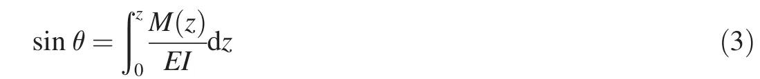
The curve length of the beam can then be calculated as

where s is the curve length of the bending beam(m),and hvis the projective height of vegetation after bending (m).Assigning P as the total load (N) uniformly distributed in flowing water over the bending vegetation and normal to the zaxis, the bending moment can be expressed as

Substituting Eq. (5) into Eq. (3) results in
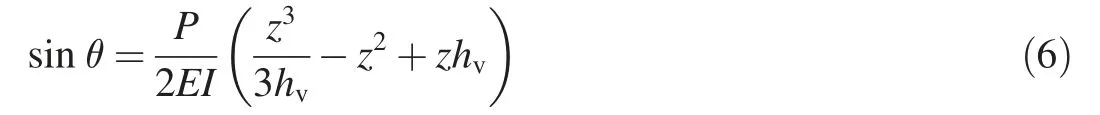
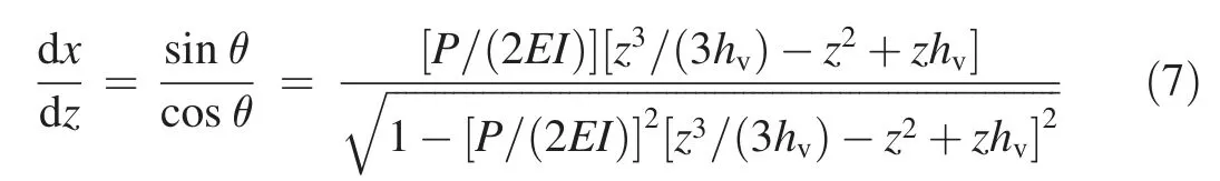
From Eqs. (4) and (6), one can further deduce
Considering force balance between the Reynolds shear stress, gravitational component, and resistance force by vegetation, the momentum equation can be written as (Huai et al., 2013)
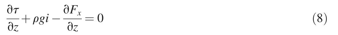
where τ is the Reynolds shear stress (N/m2), ρ is the water density (kg/m3), g is the gravitational acceleration (m/s2), i is the bed slope,and Fxis the resultant force per unit area along the x-axis (N/m2). In the vegetated zone, the Reynolds shear stress can be described as

where α is a constant; and h is the water depth above the vegetation top (m), with h = H-hv. Considering a small element of flexible vegetation in Fig.2,theoretically there are two types of forces acting on it: the drag force FD, normal to the plant stem(N/m2);and the friction force Ff,along the plant(N/m2). These forces could be calculated by the following approach proposed by Bootle (1971):

where m is the vegetation density(m-2);Afis the frontal area of the element(m2);Asis the surface area of the element(m2);D is the frontal-projected width of the stem (m), equal to the stem diameter;andCpistheperimeterofthestemcrosssection(m),and Cp=πD.For circular cylinders,ds can be described as follows:

Following Newton's Third Law, the resultant force component dFxcan be described as

To find the resultant force of vegetation in a horizontal direction, Eqs. (6) and (10)-(12) can be used in Eq. (13),creating the following formula:

Fig. 2. Bending of single flexible vegetation stem.

where H is the total flow depth (m). By substituting Eqs. (9)and (14) into Eq. (8), the vertical velocity distribution in the vegetation layer can be computed as (Huai et al., 2013)stem was taken as 0.00095 m,and Cp=0.00261 m was assumed based on the elliptical cross section.The experimental parameters are listed in Table 1.
The velocity profile comparisons are presented in Fig. 3.For comparison and validation purposes, the results are presented for densely vegetated flow cases 1.1.3 and 1.2.1 with 10000 stems per square metre, and for sparse cases 2.1.1, 3.1.1, 4.1.1, and 2.2.1 with 2500 stems per square metre. It can be observed that the analytical results are in agreement with the measured data under different vegetation densities. The measured S-shaped profile of the vegetated flow has been reproduced by the model with reasonable precision, which means that the modelling concept of combining Eqs. (15)-(17) to represent the velocity distri-
At the top of the vegetation,where z =hv,the flow velocity can be obtained as butions in different zones, i.e., vegetated and non-vegetated zones, works well. Besides, the modelled curve profiles do
The flow velocity in the free-water layer could also be expressed by the log-law as(Huai et al.,2009;Liu et al.,2012)
where uvis the velocity averaged over the vegetated layer(m/s);and u*represents the shear velocity at the top of the vegetation,with u*=
4. Results and discussion
An experimental study by Kubrak et al.(2008)was investigated for model validation in this study.In the experiments,two components of velocity,i.e.,longitudinal and transversal,were measured in a glass-walled flume with a length of 16 m and a width of 0.58 m. Cylindrical flexible stems of elliptical cross sections(with dimensions:wide diameter D1=0.00095 m and narrow diameter D2=0.0007 m)were used in their experiments to represent vegetation. The frontal-projected width D of the not show any discontinuous plot or instable spikes, and this gives confidence that the multiple modelled equations work well together. The comparison has also proven that the present model can be used to represent the longitudinal velocity distribution along flow depth with submerged flexible vegetation.
Through detailed analysis, it can be observed that the calculated results by the studied model for densely vegetated flow cases are more accurate in general,compared to sparselyvegetated flow cases.Referring to Fig.3,the main discrepancy between the calculated and measured data for sparsely vegetated flow cases occurs at the free-water layer within the nonvegetated zone,where the modelled results do not match with the measured data as closely as in the vegetated zone. This might be caused by the log-law assumption in Eq.(17),where it is suggested in some studies that the assumption should be improved and modified (Lassabatere et al., 2013; Pu, 2013).
Table 1Experimental parameters from Kubrak et al. (2008).
In terms of measurements, the sparse vegetation condition creates more space in between vegetation stems, hence promoting flexible vegetation projectile fluctuation within the experimental flow. This fluctuation movement will in turn generate a higher degree of non-linear vegetation drag and friction forces that spin off to the free-water layer, and hence affect the accuracy in the model representation. Because of this,it will be interesting to conduct a further detailed study of the drag and friction effects on the model for flow with flexible vegetation as in sections 4.1 and 4.2.
The calculated data were also compared with measurements for all six cases in terms of detailed root-mean-square errors (RMSEs) in Table 2. It can be observed that all computations give reasonable accuracy by showing RMSEs of less than 5% across the whole velocity profile when compared to the measured depth-averaged velocity.Further analysis reveals that most of the test cases with high vegetation density are more accurately modelled compared to low vegetation density cases with similar H and hv, as less space between the high dense vegetation allows its characteristics to be more easily captured by the model in Eqs. (15) and (16).
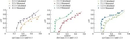
Fig. 3. Comparison of calculated and measured data for flow with flexible vegetation.

Table 2Comparison of measured and calculated results.
4.1. Sensitivityanalysisofdragcoefficientinvegetatedzone
In the presence of other neighbouring cylinders, the drag force would vary with cylinder spacing, as proven by studies of Cheng and Nguyen (2011), Kothyari et al. (2009), and Tanino and Nepf (2008). Thus, using a constant value for CDcould not give a precise estimation of the drag force by flexible vegetation since CDhas a complicated dependence on the Reynolds number, Froude number, vegetation density, and its flexibility.
According to Pope(2000),the drag force experienced by a vegetation body within a flow can be represented as

Fig. 4 illustrates the sensitivity analysis for velocity profile with changes in CD. The analysis of CDvalues between 1.2 and 1.9 was used in the suggested model to study their influence on velocity distributions. This range corresponds reasonably to the constant value of 1.4 used by Huai et al.(2013) who also studied test cases 1.2.1, 2.2.1, and 4.1.1 in Kubrak et al. (2008). Fig. 4 suggests that CDvalues used in velocity modelling should vary with flow and vegetation properties.
In most of the test cases, the measured velocity profiles fluctuate at different flow depths, which proves that the representative CDshould be non-constant.Compared to dense vegetation cases presented in Fig. 4(a) and (b), in sparsely vegetated flows (i.e., test cases 2.1.1, 2.2.1, 3.1.1, and 4.1.1 shown in Fig. 4(c)-(f)), the velocity distribution fluctuation can be observed due to the vegetation frontal vibration in the cases with flexible vegetation. These results for sparse vegetation cases have been represented poorly when CDis fixed at 1.4,as suggested by Huai et al.(2013).In short,through these findings this study cautions against adopting a constant value of CD, which is commonly suggested in the literature.
4.2. Sensitivity analysis of friction coefficient in vegetated zone
A sensitivity analysis carried out for the friction coefficient Cfis presented in Fig.5.It can be found from Fig.5(a)and(b)that there is no significant influence of Cfon the calculated velocity profiles for the dense vegetation cases 1.1.3 and 1.2.1,since the calculated velocity profiles with different Cfvalues have almost overlapped. This corresponds to the fact that the large vegetation density used in the experimental cases 1.1.3 and 1.2.1 has restricted the flexible vegetation movements.This movement restriction can create higher and more detectable vegetation friction to flow. In comparison with the dense vegetation condition, Cfshows more significant impact on the calculated velocity profiles in sparse vegetation cases 2.1.1, 2.2.1, 3.1.1, and 4.1.1 (in Fig. 5(c)-(f)).

Fig. 4. Sensitivity analysis of drag coefficient for flow with flexible vegetation.

Fig. 5. Sensitivity analysis of friction coefficient for flow with flexible vegetation.
As with the investigation of CD, Cfexhibits a more fluctuating nature in the sparsely vegetated flow cases (as shown in Fig.5(c)-(f)).In these flows,the highly fluctuating readings of velocity profiles could be represented by the non-constant Cfwith a higher accuracy, which suggests that Cfshould be characterised by a range rather than a constant value. Also,large variations used, with Cfbetween 0.1 and 1.6, need to fit the measured data,as compared to a single constant value of 0.4 suggested by Kubrak et al. (2008). This suggests that the friction force should vary by a larger range in the flow with flexible vegetation as compared to the drag force. However, the fluctuation patterns for velocity profiles, especially in the freewater zone, are not varying as much with a large range of Cfused.This further suggests a limited impact of the friction force in the non-vegetated zone, which significantly limits the influence of Cfon vegetated flow modelling. In summary, a better understanding of the Cfrange is needed for more precise velocity profile modelling in the vegetated zone.
5. Conclusions
(1) This study investigated the impacts of the drag coefficient CDand friction coefficient Cfon the flow with flexible vegetation using an analytical model based on the two-layer velocity distribution and large-deflection cantilever beam theories.
(2) The results show that CDand Cf, with their values considered to vary within certain ranges, can represent the vegetation drag and friction forces at a higher accuracy when compared to commonly used approaches that consider CDand Cfas constant values. It was also found that CDhas a more dominant influence on the velocity distribution in the flow with flexible vegetation, as compared to Cf.
(3)From a sensitivity analysis of Cfin the range of 0.1-1.6 and CDin the range of 1.2-1.9, it was found that most discrepancies between the calculated and measured velocity profiles occurred in the free-water layer of sparsely vegetated flow.This is because the sparse vegetation condition permits a larger flexible vegetation projectile fluctuation in experiments that causes greater ranges of CDand Cf, which in turn demonstrates the inaccurate assumption of constant values of CDand Cfin analytical models for calculating the velocity distribution.
 Water Science and Engineering2019年2期
- Water Science and Engineering的其它文章
- Using multi-satellite microwave remote sensing observations for retrieval of daily surface soil moisture across China
- Impacts of rainfall and catchment characteristics on bioretention cell performance
- Numerical simulation of wind-driven circulation and pollutant transport in Taihu Lake based on a quadtree grid
- Correlations between silt density index, turbidity and oxidation-reduction potential parameters in seawater reverse osmosis desalination
- River bank protection from ship-induced waves and river flow
- Possibilities and challenges of expanding dimensions of waterway downstream of Three Gorges Dam