Likelihood Ratio Tests for Homogeneity of Multiple Populations in a Parametric Family

QIN Yongsong, HUANG Meiqing

(Department of Statistics, Guangxi Normal University, Guilin 541004)

Abstract: The test for the homogeneity of several populations is a common issue in many application fields. The well-known results related to this issue include the analysis of variance (ANOVA) for normal populations and the Kruskal Wallis Test (KWT)for nonparametric populations, but there is no general result on the test for the homogeneity of parametric populations. In this paper, the likelihood ratio test (LRT)statistic is constructed to test for the homogeneity of several populations which are the members of a parametric family. It is shown that under some regularity conditions and the null hypothesis all distribution functions of the populations are the same, and the limiting distribution of the LRT statistic is chi-squared distribution.This result fills in a gap between ANOVA for normal populations and KWT for nonparametric populations.

Keywords: parametric family; test of homogeneity; likelihood ratio test

1 Introduction

It is a common and classic issue in practice to decide whether serval samples should be regarded as coming from the same population. This is a problem of testing homogeneity in statistics. Two well known testing methods have been used to address this issue. They are the analysis of variance(ANOVA)for normal populations and Kruskal-Wallis test (KWT) for nonparametric populations. Now a new problem arises: what kind of testing method should be used if serval samples comes from the same parametric (not limited to normal distribution) family? ANOVA can not be used here as it is only efficient for normal distribution families. Since parametric structures are not employed, KWT may be used but less powerful than a suitable parametric method.

In this paper, the likelihood ratio test (LRT) statistic is constructed for testing the homogeneity of several populations which are the members of a parametric family.Under some regularity conditions and under the null hypothesis that all distribution functions of the populations are the same, it is shown that the limiting distribution of the LRT is chi-squared distribution. This result fills in a gap between the well known known tests of homogeneity: ANOVA and KWT. Due to the well known merit of likelihood method,we can expect the good performance of the method proposed in this paper, which will be presented by our extensive simulation studies. In nonparametric settings, KWT provides tests of the null hypothesis that independent samples from two or more groups come from identical populations, which requires less assumptions about the distribution of the data than that in this paper. However, KWT may be less powerful than the LRT studied in this paper when parametric structures are available.We will conduct a comprehensive comparison between LRT and KWT in the simulation section.

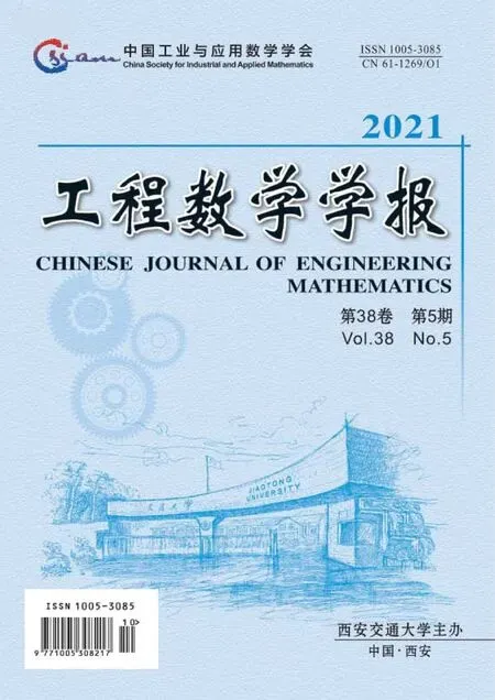
Refer to Lehmann[1]for the theory and applications of KWT.Here we briefly state the definition of the KWT and its limiting distribution. Arrange the data of all samples in a single series in ascending order. Assign rank to them in ascending order. In the case of a repeated value,or a tie,assign ranks to them by averaging their rank position.The KWT statistic forkindependent samples, each of sizeniis

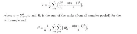
whereRijis the rank (from all samples pooled) of thej-th observation in thei-th sample. The null hypothesis of this test is that allkdistribution functions are equal.It is shown, under the null hypothesis and some regularity conditions, that

The rest of the paper is organized as follows. The main results of this paper are presented in section 2. Results of a simulation study on the finite sample performance of the LRT are reported in section 3. The proof of the main results is presented in section 4.

2 Main results

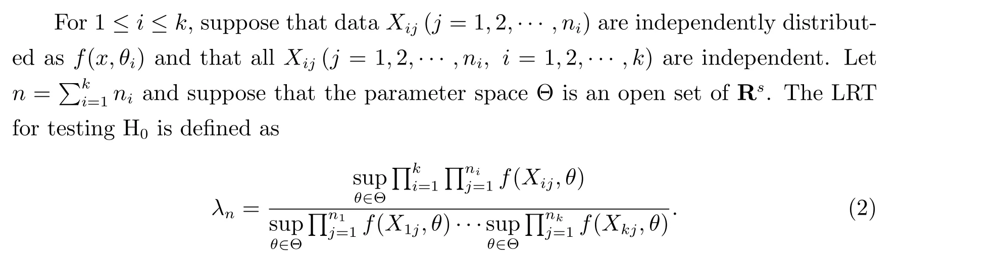
Suppose that there arek(k ≥2)populations and thei-th population has probability density function (or mass function)f(x,θi)(1≤i ≤k) (with respect to aσ-finite measureμ), whereθi ∈Θ⊆Rs(s ≥1),1≤i ≤k, the form offis known,θiare unknown parameter vectors, and Θ is the parameter space. Consider the hypotheses

This test for homogeneity arises quite often. For example, in the comparison of a number of different treatments, processes, varieties, or locations, one wishes to test whether these differences have any effect on a outcome.

The LRT rejects H0for large values of-2 logλn.

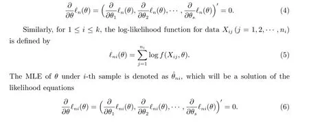
Under H0, the log-likelihood function is defined by

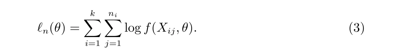
Suppose that there is a unique ˆθnwhich maximizesℓn(θ). Then ˆθnis called the maximum likelihood estimator (MLE) ofθ. Suppose that, in addition,ℓn(θ) is differentiable inθ. Then ˆθnwill be a solution of the likelihood equations

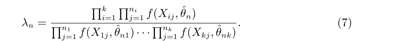
We assume that all ˆθn,ˆθniare consistent estimators ofθas min1≤i≤k ni →∞. These are commonly used settings in studying the large sample properties of the MLE[2,3].Under these settings,λncan be re-written as

LetXbe the population with distributionf(x,θ). To obtain the asymptotic distribution ofλn, we need some more regularity conditions as follows[2]:

(A) There exists an open subset Θ0of Θ containing the true parameter pointθ0such that for almost allx,the densityf(x,θ)admits all third derivatives(∂3/∂θi∂θj∂θl)f(x,θ) for allθ ∈Θ0;

(B) The first and second logarithmic derivatives offsatisfy the equations

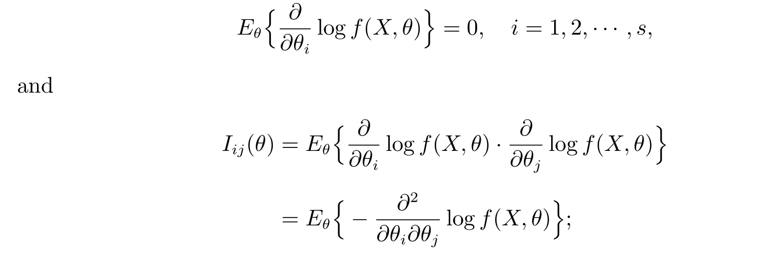
(C) Thes×sFisher information matrixI(θ)=(Iij(θ)) is positive definite for allθin Θ0;

(D) For allθ ∈Θ0and alli, j, l, there exist functionsMijlsuch that

whereEθ0{Mijl(X)}＜∞.

We now state the main results in this paper.

Theorem 1 Suppose that Assumptions (A)-(D) are satisfied. Then, under H0,as min1≤i≤k ni →∞,

Remark 1 If we useλnin (7), in stead of (2), as the original definition, where ˆθn,ˆθniare the roots of related likelihood equations, then Theorem 1 still holds true.This can be seen from the proof of Theorems 1. In other words, ˆθn,ˆθnido not need to be the MLEs to have the results of Theorem 1.

Remark 2 There is no doubt that ANOVA should be used in testing homogeneity for normal families. On the other hand, in testing homogeneity for non-normal parametric families, LRT is recommended. However, if the regularity conditions stated above are not satisfied, the limiting distribution of the LRT may not be the stated distribution above and the results in this paper can not be used in this case.

Remark 3 The regularity conditions (A)-(D) are the same as the well known Wilks theorem for the LRT used to test the null hypothesis that the parametric vector equals to a given value in a one sample parametric family[3,4]. However, the problem addressed in this paper is different with that in Wilks theorem. As to the method of derivations of our main results, Lemma 1 below is a new result that is used in this paper. In addition, the method in proving Wilks theorem is also used in this paper. Surprisingly, to the best of our knowledge, there is few references on the test for homogeneity of multiple populations in a parametric family.

3 Simulation results

Several commonly used parametric families were used in our simulations,which are shown in Table 1.

Table 1 Parametric families investigated in simulations

In the whole simulations,θ0was used to denote the true parameter point of a parameter vectorθ. To save space, only one true parameter point of a parameter vector was considered and only comparison of 3 populations were conducted.

From every family, we generated 2000 samples with various sample sizes and compared the sample quantiles of-2 logλnwith the quantities of related chi-squared random variables stated in Theorem 1, which were illustrated in Figures 1 to 4.

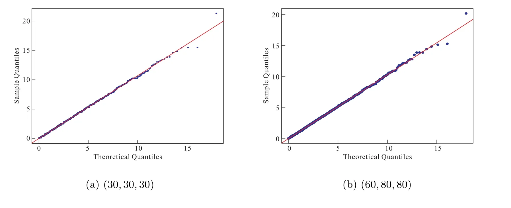
Figure 1 Bernoulli: Q-Q plots of -2 log λn against χ22 under p0 =1/4

Figure 2 Poisson: Q-Q plots of -2 log λn against χ22 under λ0 =1

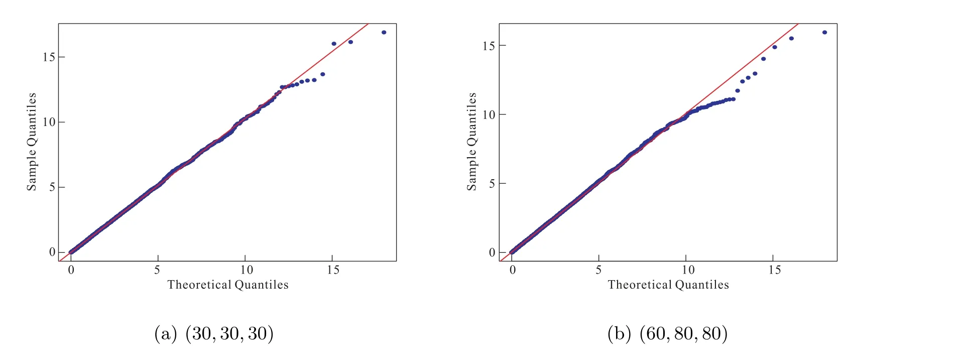
Figure 3 Exponential: Q-Q plots of -2 log λn against χ22 under θ0 =1

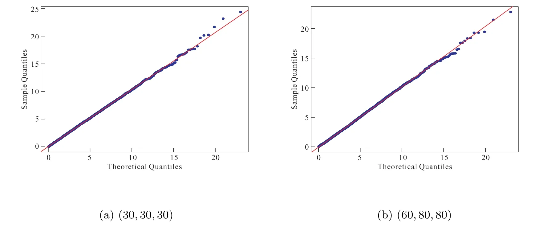
Figure 4 Gamma: Q-Q plots of -2 log λn against χ24 under (a0,b0)=(1,1)

From these results, it is seen that the simulated percentiles are quite close to theoretic ones even for moderate sample sizes, with better agreement as sample sizes increase.

Further, the simulated rejection rates of LRT and KWT under several alternatives were compared,using 2000 Monte Carlo trials with various sample sizes. The significant level was always set as 0.05 in the simulations. The results of these comparisons were reported in Table 2. It is understandable, according to Remark 2, that normal families and ANOVA are not included in the simulations. From these simulation results, it can be seen that the simulated powers are quite well for both tests and LRT performs better than KWT.

Table 2 Rejection rates under sample sizes (30,30,30) and (50,60,70) and different alternatives indicated in terms of parameters

4 Proofs

By assumption (D) and the law of large numbers, one can show, under H0andθ=θ0,that

By the law of large numbers, we haveH=-I(θ0)+op(1).We thus have (9).

Now expandingℓn(ˆθn) aboutθ0, we have

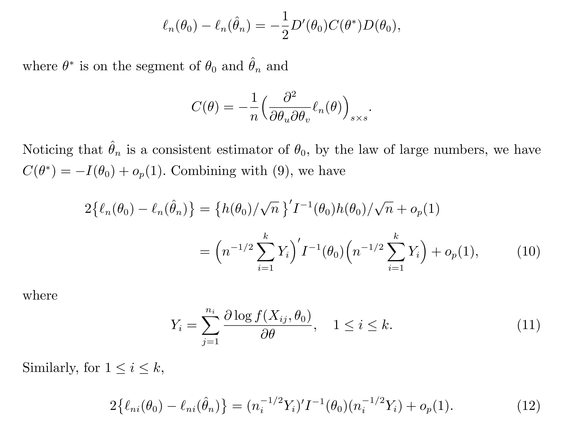
Notice that

By the central limiting theorem,

We thus have Theorem 1.