
Recent Trends in Satellite-Derived Chlorophyll and Aerosol Optical Depth Together with Simulated Dimethylsulfide in the Eastern China Marginal Seas
2022-02-24 08:23QUBoandGABRICAlbert
QU Bo, and GABRIC Albert J.
Recent Trends in Satellite-Derived Chlorophyll and Aerosol Optical Depth Together with Simulated Dimethylsulfide in the Eastern China Marginal Seas
QU Bo1), *, and GABRIC Albert J.2)
1) School of Science, Nantong University, Nantong 266000, China 2) School of Environment and Science,Griffith University, Brisbane, QLD, Australia
The biogenic compound dimethylsulfide (DMS) produced by a range of marine biota is the major natural source of reduced sulfur to the atmosphere and plays a major role in the formation and evolution of aerosols, potentially affecting climate. The spatio-temporal distribution of satellite-derived chlorophyll_(CHL) and aerosol optical depth (AOD) for the recent years (2011–2019) in the Eastern China Marginal Seas (ECMS) (25˚–40˚N, 120˚–130˚E) are studied. The seasonal CHL peaks occurred during late April and the CHL distribution displays a clear zonal gradient. Elevated CHL was also observed along the northern and western coastlines during summer and winter seasons. Trend analysis shows that mean CHL decreases by about 10% over the 9-year study period, while AOD was higher in south and lower in north during summertime. A genetic algorithm technique is used to calibrate the key model parameters and simulations are carried out for 2015, a year when field data was available. Our simulation results show that DMS seawater concentration ranges from 1.56 to 5.88nmolL−1with a mean value of 2.76nmolL−1. DMS sea-air flux ranges from 2.66 to 5.00mmolm−2d−1with mean of 3.80mmolm−2d−1. Positive correlations of about 0.5 between CHL and AOD were found in the study region, with higher correlations along the coasts of Jiangsu and Zhejiang Provinces. The elevated CHL concentration along the west coast is correlated with increased sea-water concentrations of DMS in the region. Our results suggest a possible influence of DMS-derived aerosol in the local ECMS atmosphere, especially along the western coastline of ECMS.
dimethylsulfide sea-to-air flux; chlorophyll-; aerosol optical depth; biogeochemical model; Eastern China Marginal Seas
1 Introduction
The Eastern China Marginal Seas(ECMS) is one of the largest semi-enclosed seas on the western rim of the Pacific Ocean. It currently acts as a net sink of atmospheric CO2exporting a significant amount of organic carbon to the North Pacific (Chen., 2004) . The southwest monsoon that prevails in summer acts together with the northward Taiwan Warm Current and China Coastal Current to cause the coastal upwelling (Chen., 2004).
Red tides are reported frequently occurred around the ECMS due to anthropogenic nutrient enrichment of the coastal waters on the western side (Tang., 2006; Kim., 2011; Mackey., 2017). One of the world’s largest rivers, the Changjiang River discharges to the East China Sea and has led to eutrophication and periodic red tides in adjacent coastal waters. Kim. (2011) found that the relative abundance of nitrate (N) over phosphorus (P) has increased since year 1980 in the ECMS. The in-crease in N availability is driven by deposition of nitrogen from atmospheric sources, with riverine nitrogen loading equally important. Those input sources have switched phytoplankton growth in the study region from being N- limited to P-limited, especially in the area located downstream of the Changjiang River plume with P-limitation especially serious in South China Sea (the southern part of our study region). The Taiwan Strait (TS) transports an order of magnitude more carbon and a factor of two more phosphate to the East China Sea (ECS) than the Chang- jiang River does (Huang., 2019). The surface N and P concentrations in the TS can be up to 15 times higher in winter than in summer due to insufficient solar radiance and colder temperature during wintertime. Therefore, the supply of P to the ECMS is the main factor that controls phytoplankton dynamics in the region.
Phytoplankton biomass (indicated by CHL) exhibits higher concentrations in the western coast of study region compared with the east part of the area towards open sea, as reported by Kong. (2019). CHL had an increased trend in the vicinity of the Changjiang River mouth and a decreased trend in the southeastern of ECS which can be attributed to anthropogenic nutrient enrichment and war- ming (Kong., 2019). Diatoms dominate the phytoplankton community in summer and autumn and dinoflagellates are the most abundant species in winter and spring (Xu., 2016, Liu., 2019). The contribution of phytoplankton communities in the EMCS are dominated by microphytoplankton or nanophytoplankton. During summer time, their contributions are higher than 70% in the coastal waters and less than 30% in the off- shelf waters (Liu., 2019).
The mixed layer depth, the light irradiance and the supply of nutrients are all critical driving forces for ecosystem dynamics in the upper ocean (Cropp., 2004). Phytoplankton blooms are also influenced by sea surface temperature (SST) and wind speed (WIND), especially before and during blooming season (Qu and Liu, 2020). The deepening of the mixed layer brings new nutrient to surface waters and the stratification of the surface waters provide phytoplankton an idea conditions for initiation of a phytoplankton bloom (Doney., 1996). Shallowing of mixed layer depth (MLD) in spring-summer can enhance phytoplankton biomass production.
1.1 Biogeochemical Modeling of DMS
As the main volatile sulfur species emanating from the oceans, DMS plays a significant role in the atmospheric sulfur cycle (Bates., 1992). DMS is derived from its precursor compound dimethylsulfoniopropionate (DMSP) which is synthesized in the cells of phytoplankton and other marine organisms. The so-called CLAW hypothesis (Charlson., 1987) proposed that as they warmed the global oceans would produce an increase in biogenic sulfate aerosol, leading to an increase in the number of cloud condensation nuclei (CCN), and changes to cloud microphysics. Ultimately the CLAW hypothesis suggested the possibility of bio-regulation of climate (Nunes-Neto., 2011). Although still debated, some modeling studies sug- gest that when DMS emissions are doubled in an atmospheric sulfur-climate model, there is a 25% reduction in the indirect radiative forcing due to anthropogenic sulfate aerosols (Jones., 2001).
DMS is produced by the marine microbial food weba complex suite of biological and chemical processes (Simó, 2004). These processes include DMSP lyases produced by phytoplankton and bacteria, the breakage of phytoplankton cells as a result of zooplankton grazing, viral attack and autolysis releases of DMSP (Simó, 2004; Stefels., 2007). Galí and Simó (2015) indicate that in the upper ocean about 90% of dissolved DMS is consumed by bacterial oxidation and UV-driven photolysis, and only 10% is emitted to the atmosphere through ventilation.
Global DMS climatologies from the study of Kettle and Andreae (1999) and Kettle and Andreae (2000) have been compiled with a database of over 15000 DMS measurements. Several authors have attempted to derive empirical relationships between DMS and other environmental parameters. Anderson. (2001) chose to use a simple empirical relationship to compute DMS from CHL, light and nutrients. Their result yields overestimate DMS concentration in the high latitude and underestimate DMS in low DMS area (Belviso., 2004). An empirical relationship between CHL, MLD and DMS are derived by Simó and Dachs (2002) (SD algorithm). Using the SD algorithm, DMS concentration is underestimated probably because of the weight they gave to deep mixed layers in winter. The two steps ratio restriction for CHL/MLD is preferable for the equatorial Pacific zone and cannot accurately predict the substantial variability in other regions (Belviso., 2004).
A depth-averaged biogeochemical DMS model G93 is used here to calculate the DMS concentration using a ran- ge of satellite derived data in EMCS region for year 2015. A genetic algorithm (GA) (Holland, 1975) technique is used to calibrate the CHL and DMS related main parame- ters in the G93 model. Sensitive analysis is carried out be- fore the calibrations. Regional DMS sea-air fluxes are calculated and compared with the field data and those calculated using the SD algorithm (Simó and Dachs, 2002).
2 Methods
2.1 Satellite Data
The study region is in the ECMS (120˚–130˚E, 25˚–40˚N) (Fig.1) and the study period is 2011–2019. The DMS modeling period is within year 2015, when the field data is available from OUC. CHL and AOD 8-day mean satellite images are retrieved from Giovanni, NASA open data portal (https://giovanni.gsfc.nasa.gov/giovanni/). CHL MODISA_L3m_CHL_8d_4km_v2018 is chosen for CHL 8-day data. CHL images are produced by NASA Earth Data in the Giovanni website (https://giovanni.gsfc.nasa. gov/giovanni/, The Bridge Between Data and Science v 4.35). MODISA_L3m_RRS_8d_4km_v2018 is chosen for the AOD 8-day data. WIND and SST were retrieved from ftp://ftp.remss.com/windsat/bmaps_v07.0.1/weeks/.Mixed Layer Depth (MLD) is obtained from http://oregon.iarc. uaf.edu/dbaccess.html where the depth varying temperature CDT (Climate Data Tool) is obtained. The MLD is then defined by the vertical depth of the temperature difference of 0.5 degree. Cloud cover (CLD) monthly mean data is obtained from https://acdisc.gesdisc.eosdis.nasa. gov/data/Aqua_AIRS_Level3/AIRX3STM.006/.
2.2 The DMS Model
The structure of the depth-averaged G93 model is a food web comprehensive model and is time-dependent with state variables averaged vertically over the MLD. The model has been described in detail by Gabric. (2001). The equations of state of the depth averaged G93 model are given by Eqs. (1)–(5) (Gabric., 1999; Ga- bric., 1993), where,represents the generic phytoplankton,is the zooplankton andis the dissolved nitrate. Total mass is indicated byo=, whereo is the initial nutrient at the start of the simulation. All of state variable initial values are averaged over the mixed layer.
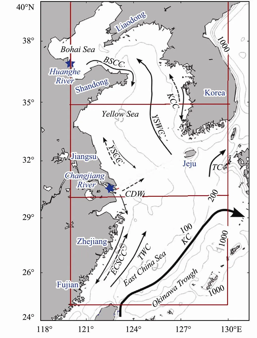
Fig.1 Surface circulation patterns and bathymetry in the study region of the ECMS (updated based on Zeng et al. (2017)). Study region is the area inside the dark red rectangular frame. Three subregions are divided for Bohai Sea, Yellow Sea and East China Sea. BSCC, Bohai Sea Coastal Current; KCC, Korean Coastal Current; YSWC, Yellow Sea Warm Current; YSCC, Yellow Sea Coastal Current; CDW, Changjiang River Diluted Water; ECSCC, East China Sea Coastal Current; TWC, Taiwan Warm Current; TC, Tsushima Current.Gray contours are 50, 100, and 1000m isobaths. Blue stars indicate the Changjiang River and Huanghe River Mouths.
The processes included in the cycling of DMS are described by the following differential equation:
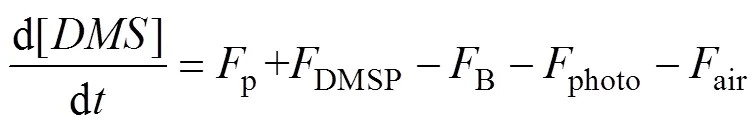
Herepis the release of DMS from phytoplankton cells,DMSPis the production of DMS from DMSP,Bis the loss of DMS by microbial consumption,photois the photolysis loss, andairis the loss due to ventilation to the atmosphere. The terms on the right hand of Eq. (1) are discussed in more detail by Gabric. (2001).
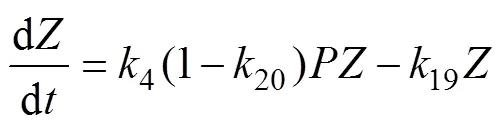
The G93 model includes two coupled sub-models. The PZN sub-model is described by Eqs. (2) to (4):
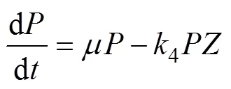

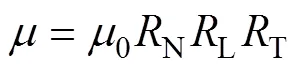
whereis phytoplankton nitrate-specific growth rate. It is limited by nutrient availability (N), light (L) and temperature (T):
The sulfur sub-model is described by the Eqs. (6)–(7):
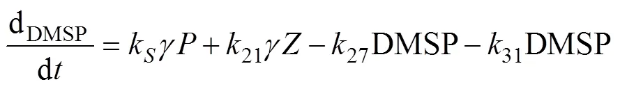
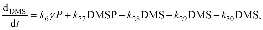
whereis the algal cell content of DMSP, which is spe- cies-specific.
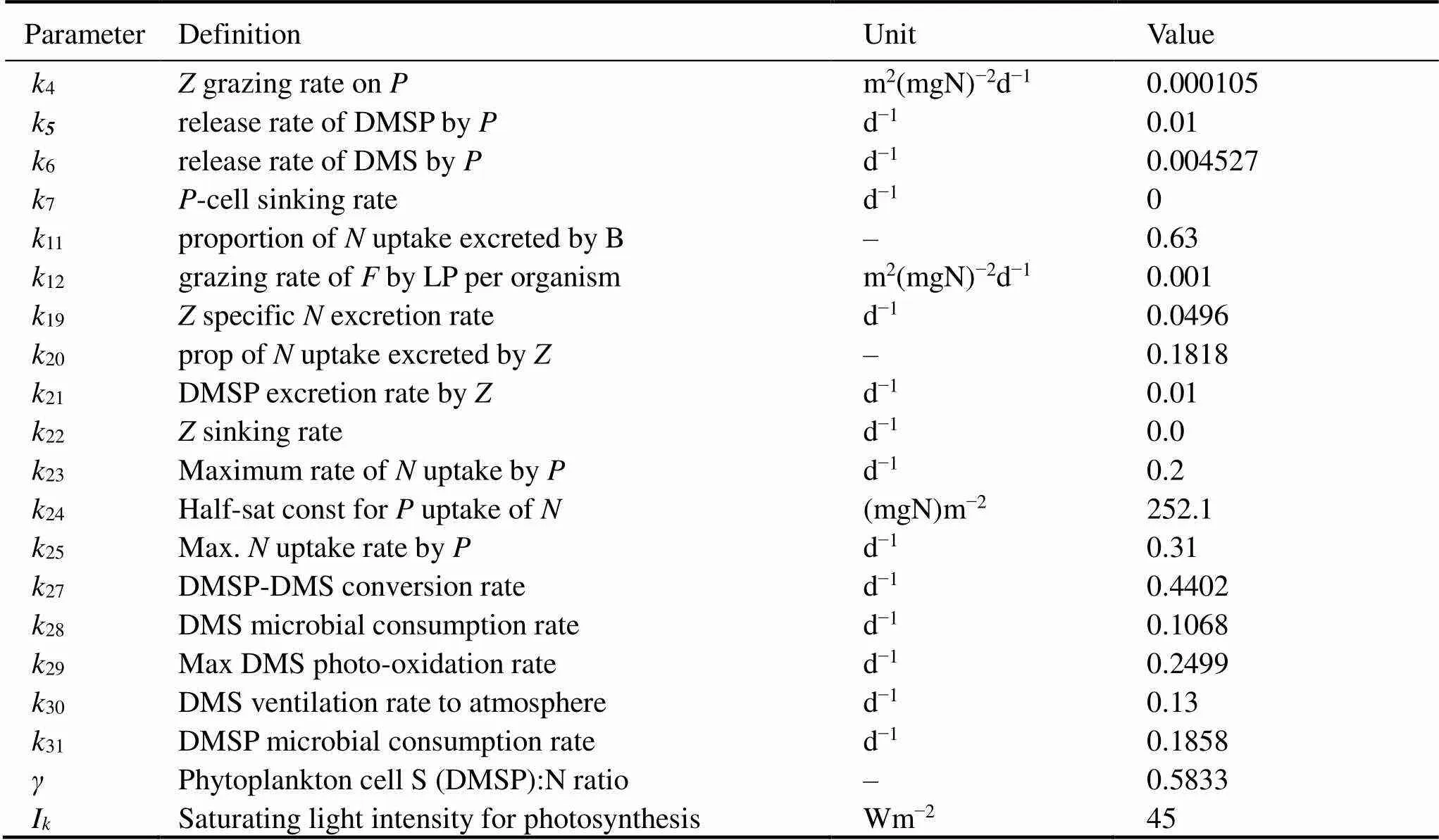
Table 1 Definition of the model parameters and input values after calibrations
The definition of the model parameter and their input values are given in Table 1, based on the values in Gabric. (1999), which focused on the Barents Sea.
Implementation of the G93 model requires knowledge of a substantial number of biological rate constants, most of which are not routinely measured. The key parameter values need to be calibrated for the ECMS study region. The ratios of carbon and nitrogen by weight: C:N ratio is set to be 8.5 and according to Liu. (2019) (who suggested the ratio is within 2.4–6.5), and Liu (1998) (who suggested the ratio is within 4.02–26.91 with mean ratio of 7.63) in the ECS region. The ratio of C: CHL is set to be 40 based on Chang. (2003) (who suggested the ratio of C:CHL is within 13–92.8 in ECS coastal waters). The model fluxes are defined in Table 2 (Gabric., 1999).
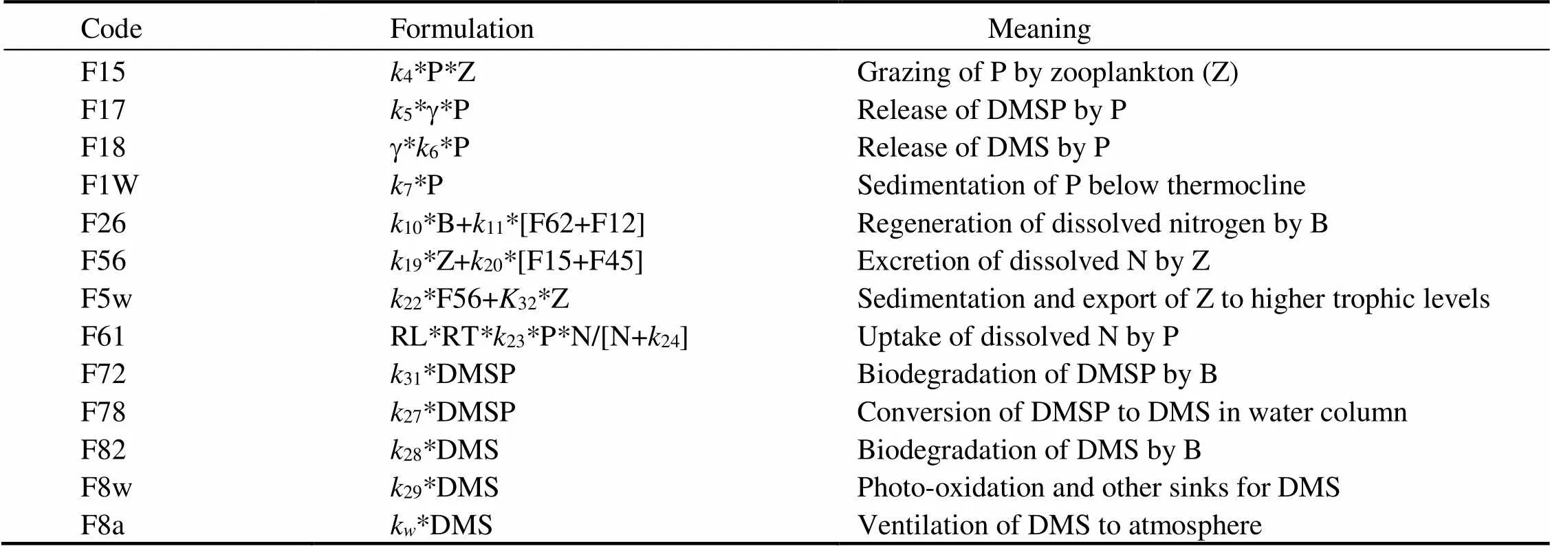
Table 2 Definition of model fluxes
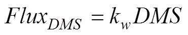
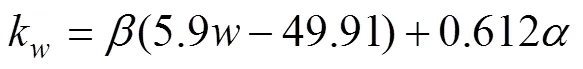
The flux of DMS from sea to the atmosphere is calculated as the product of DMS concentration and the sea- to-air DMS transfer velocityk:
The transfer velocitykis calculated in terms of WIND (noted as)at 10m above sea surface and SST (Liss and Merlivat, 1986):
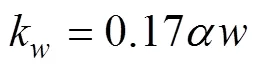
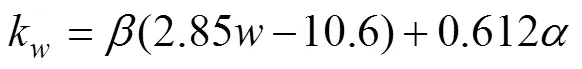

In ECMS, there was only little ice cover (less than 7%), so we ignored sea ice effects in the model simulations. The impact of effective wind fetch and the wave climate are also ignored in the model.
3 Results
The study region is divided into three five-degree zonal subregions: northern region (Bohai Sea: 35˚–40˚N); mid- dle region (Yellow Sea: 30˚–35˚N) and southern region: (East China Sea: 25˚–30˚N) (Fig.1).
3.1 The CHL and AOD Distributions
Fig.2 shows the mean CHL over the period 2011–2019 compared with that in year 2015. Year 2015 had a slightly later peak CHL on 23 April compared to the decadal mean. In general, year 2015 had a similar CHL profile to other years.
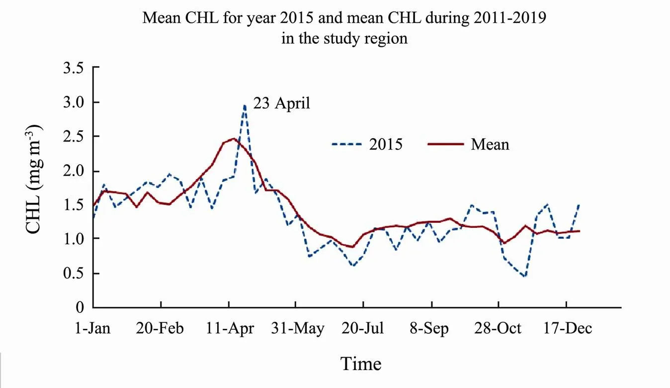
Fig.2 Spatial mean CHL time series for year 2015 (dash line) compared with the time-average for 2011–2019 in the study region (solid line).
Fig.3 shows the mean surface CHL during March, April, August and October of 2015. Higher concentration of CHL started in the northwest region (Bohai Sea) and coastal regions in both western and eastern boundaries in early year of 2015, spread offshore in all northern and most of the middle regions (Bohai and Yellow Seas) by late of April reaching a peak by 23 April). During summer, CHL is reduced especially in the offshore part of the study region. By August, CHL peaked along the east coast of Bohai Sea and west coast of ECS and southern coast of Yellow Sea. However, after September, a second peak of CHL appeared along all the coastal regions of EMCS, but decrease to a minimum by mid-November (not show in the figures).
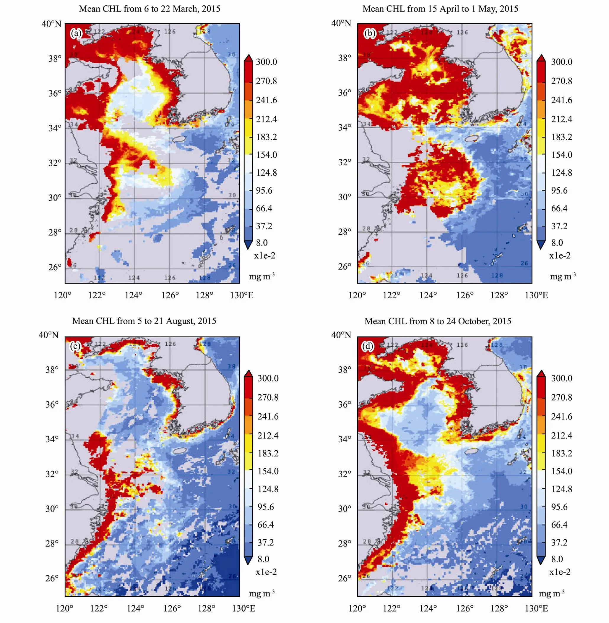
Fig.3 Time mean images of CHL for the 4 time periods in year 2015. (a), 6 to 22 March; (b), 15 April to 1 May; (c), 5 to 21 August; (d), 8 to 24 October, in the study region.
Mean CHL time series in year 2015 for the different sub-regions is shown in Fig.4. The northern region had higher profile than other two subregions. However, middle region had highest CHL peak in the 30 March. Nor- thern region reached to CHL peaks in the 15 April and the 9 May. Southern region had lowest CHL in general, with peak arrived in the 1st May. Northern region had higher winter CHL profiles apart from the end of March..
The decadal mean time series of CHL for the period 2011–2019 is plotted together with the mean of AOD for the same time period (Fig.5). CHL peaked on 15 April and reached a minimum around 12 July. The AOD peak was around 26 February, stayed high during March, and started to decrease after April. The correlation of CHL and AOD is around 0.5 for the 9-year time period. The mean correlations between CHL and AOD in year 2015 are shown in Fig.6. High correlations are evident along the west coast of the Yellow Sea and in Jiangsu and Zhejiang Provinces coastal waters. The positive correlation region is stronger in the southern region, with negative correlations in the northern region and positive along the western coast of the southern region.
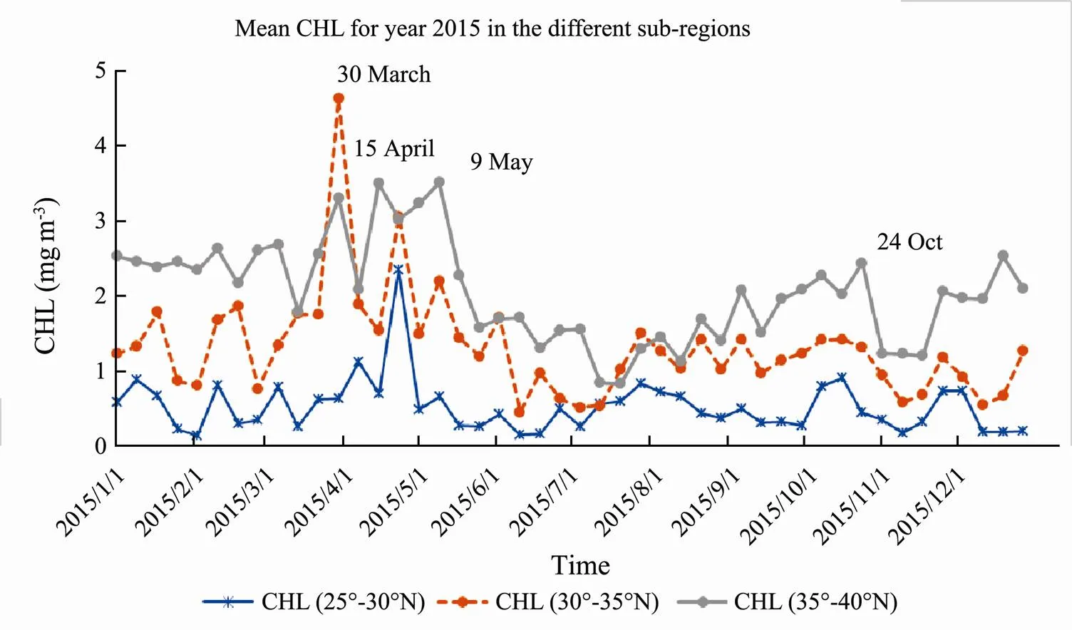
Fig.4 MODIS CHL mean time series in the sub-regions in 2015.
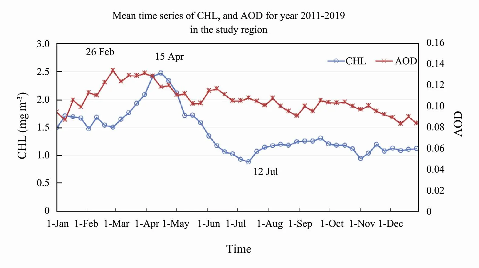
Fig.5 Mean time series of CHL and AOD for year 2011–2019 in the study region.
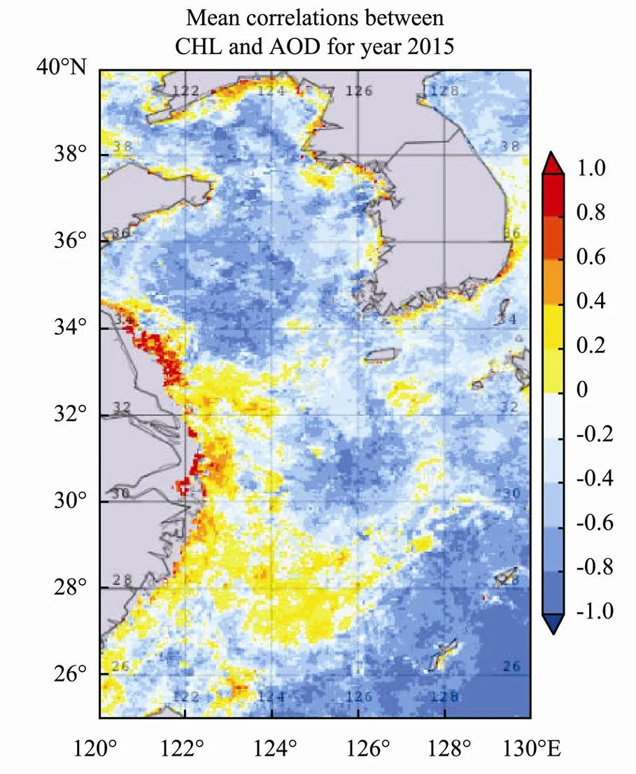
Fig.6 The correlation between CHL and AOD for 2015.
The trend in annual mean CHL for the study period is shown in Fig.7. CHL decreased 3.66% for the whole time period, decreased more than 10% during spring time (March–May) and decreased 7.91% during autumn time (August and October). Annual mean AOD decreased insignificantly (only 0.07%) for the whole time period, decreased 0.11% and 0.06% during spring time and autumn time respectively (not shown in the figure).
Year 2015 AOD spatial mean images for the 4 different time periods are shown in Fig.8. AOD was higher in the western coast of Yellow Sea in February. And gradually spread out towards eastern region and reached to its peak in the middle of March. AOD reduced by April especially in the western coast. However, in July, the higher AOD occurred more in the southern region. AOD is significant decreased by summertime in the northern region.
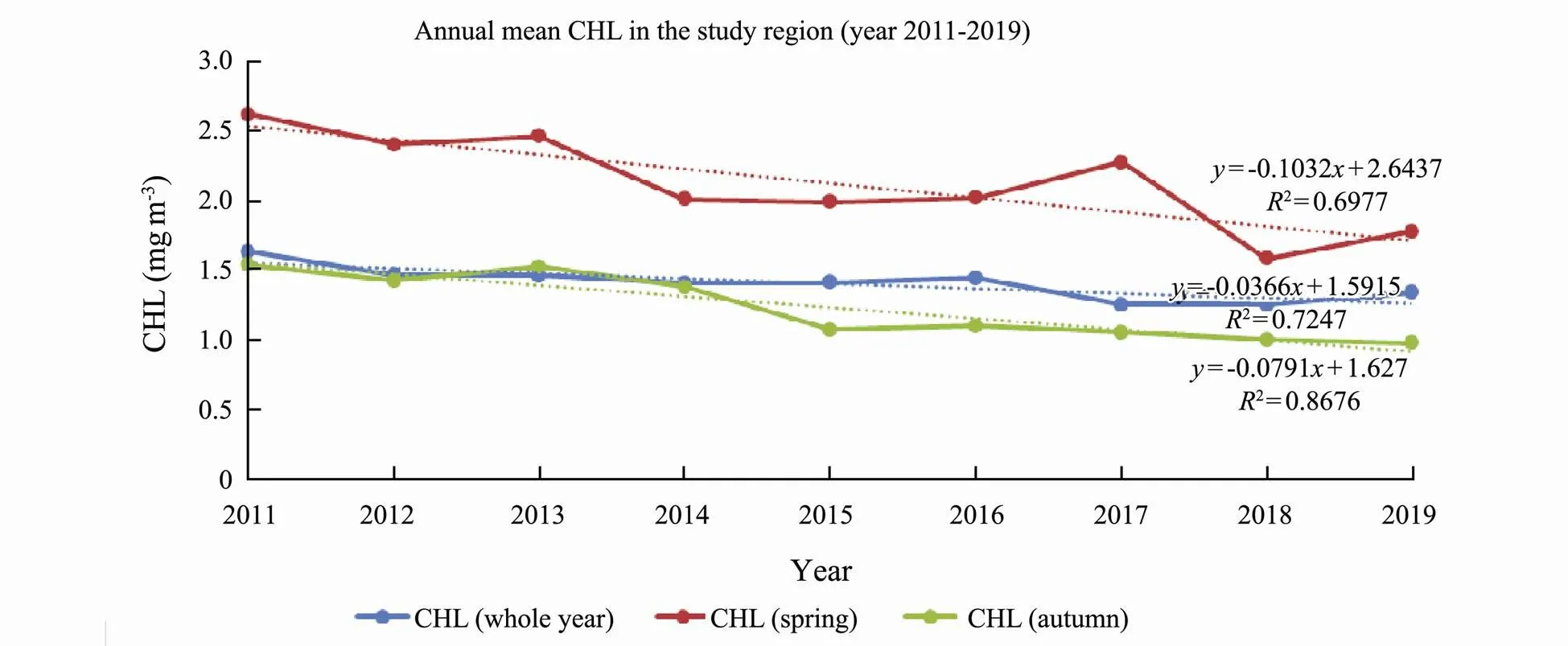
Fig.7 MODIS CHL annual mean in the study region for year 2011–2019 for the whole year, spring time and autumn time periods.
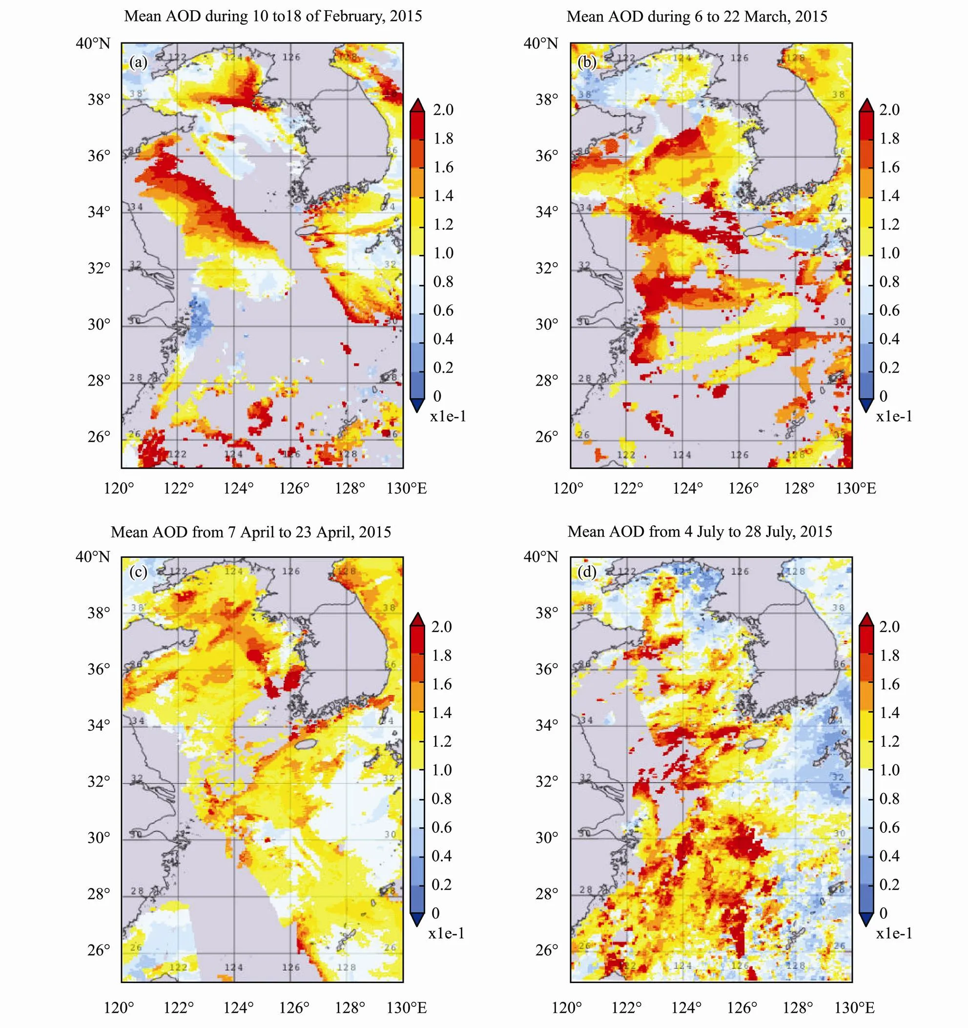
Fig.8 Time mean images of AOD for the 4 time periods in year 2015: (a),10 to 18 February; (b),6 to 22 March; (c), 7 to 23 April; (d), 4 to 28 July.
3.2 Model Calibration and Simulations
The G93 model input files contains the parameters setting and the monthly mean meteorological forcings (including SST, CLD, WIND, and MLD). Ice cover is ignored here. A sensitivity analysis is carried out before key parameter calibration. We used similar sensitivity analysis method as described in previous work (Qu., 2016, Qu., 2017), changing one parameter at a time, while fixing all other parameter values. The simulation is run using the original parameter value varied by plus or minus 20% . For the PZN submodel, the most sensitive parameter is23(maximum rate ofuptake by P), with19(specific N excretion rate) and4(grazing rate on P) the second and third most sensitive parameters. For DMS submodel, the most sensitive parameter is γ (phytoplankton cell S (DMSP): N ratio). The second sensitive parameter is28(DMS microbial consumption rate) with31(DMSP microbial consumption rate) the third most sensitive parameters.
The monthly mean meteorological forcings in year 2015 are calculated according to the satellite derived data (Fig.9). CLD is mainly within 50%–60% in the study region. October had less cloud (around 40%) than other months. SST had its peak in August and reached to more than 27℃. MLD had its peak in March and reached as deep as 145m. The summer MLD had its valley in July and only reached to the depth of 20m. WIND was winter high and summer low. Average WIND range is within 5–10ms−1.
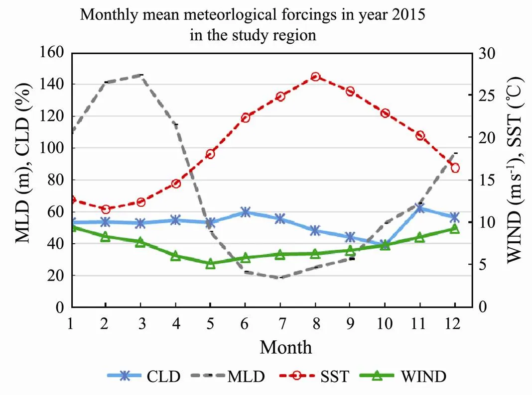
Fig.9 Monthly mean meteorological forcings (CLD, MLD, SST and WIND) in year 2015 in the study region.
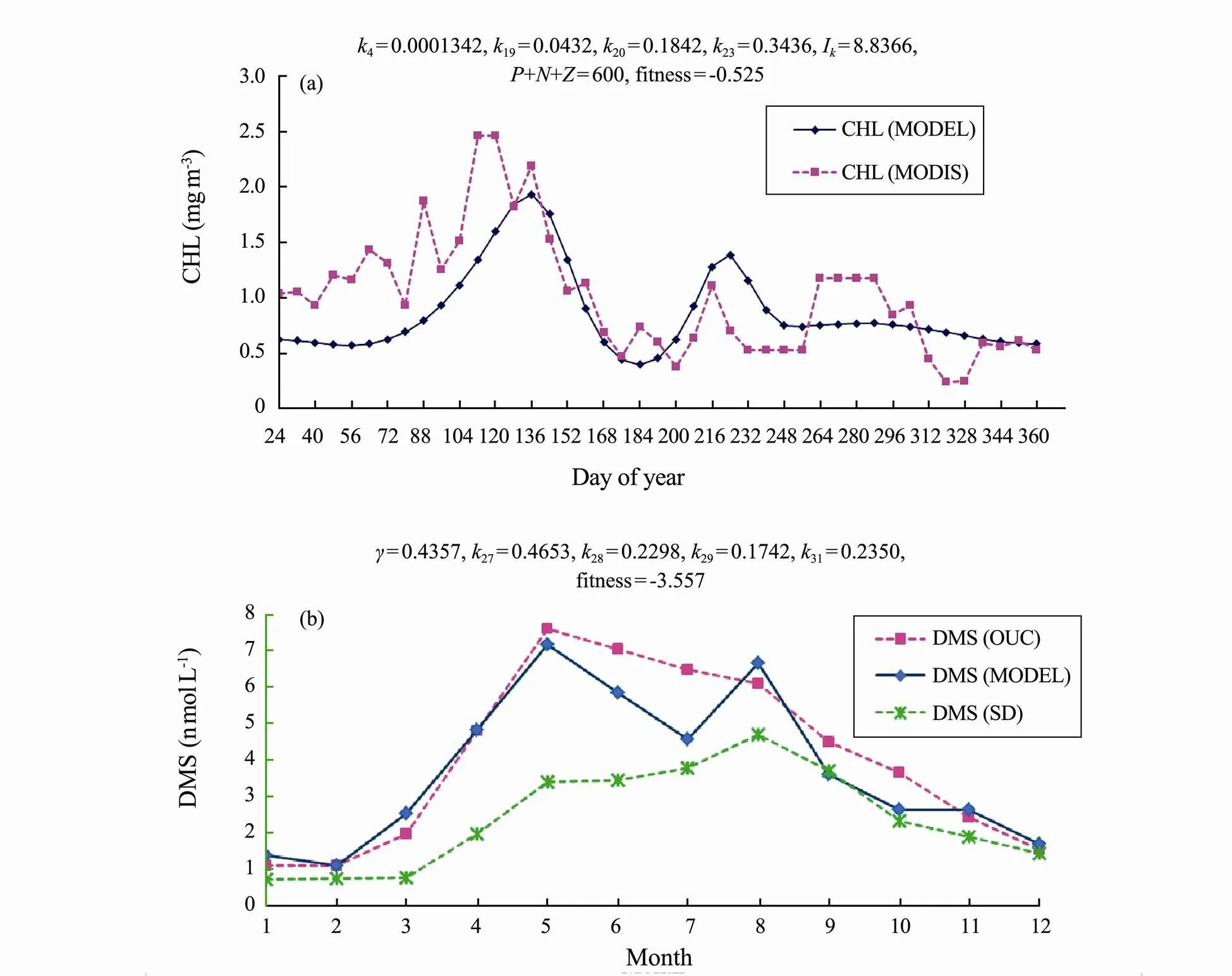
Fig.10 Genetic Algorithm calibration results for key parameters in year 2015 in the study region with (a), CHL MODIS satellite data; (b), DMS observation field data from OUC and compared with calculated DMS from Simó and Dachs formula.
Beforerunning the G93 model, the sensitive model parameters need to be adjusted through a calibration process. A Genetic Algorithm (GA) technique (Holland, 1975) is used for the parameter estimation. The fitness function is used to minimize the differences of observed data and the model simulated data. It has a process of natural selection and mixed with process of selection, crossover and mutation, the offspring is then produced which inherit the characteristics of the parents and have better fitness. The process keeps on iterating until the fitness function has no significant improvement. Here we adopted a fitness function using the time square root (2) function in order to minimize the differences between observed data and mo- del simulated data. The closer to zero, the better the fitness is. When fitness value had no longer improve, we could manually stop the iteration process and all relevant parameters values are then obtained.
The key parameter calibration are carried out in two stages: In the first stage is PZN related key parameter calibration. The satellite derived mean CHL time series is used as the observation data for the fitness function calculation. The second stage involves calibration of the DMS related sensitive parameters. The observed data used in fitness function is based on the OUC provided DMS field data. The six most sensitive CHL related parameters (4,19,20,23,Iando (=)) are calibrated first, followed by the five DMS related parameters (27,28,29,31and) calibrations. In order to generate a spring bloom, the total nutrient value was set to a reasonably large number (Gabric., 2005; Qu and Gabric, 2010; Qu., 2016).
Fig.10 shows the model calibration results for both CHL related key parameters (Fig.10(a)) and DMS related key parameters (Fig.10(b)) (blue line) comparing to the field data (MODIS satellite data as CHL observation data and OUC field data as DMS observation data) (pink line). The calculated DMS monthly profile according to the SD method is also compared (Fig.10(b)). The final key parameter values are listed in the figure’s captions. The fitness functions are 0.525 and −3.557, respectively, for CHL GA and DMS GA calibrations. Fig.10(b) shows clearly that our model simulation result is more close to the OUC field data comparing to the result used SD method. SD method tends to underestimate the DMS values.
CHL GA calibration had the peak of model simulation matched MODIS satellite data quite well (Fig.10(a)), although there was half month gap between the simulated data and the MODIS data. The first peak was in late March (MODIS data) and middle April (Model data). There was a second peak in early July. DMS had both peaks in May (for model simulation result and OUC field data) (Fig.10(b)). Model simulation shows the second peak in August, which is the peak of calculated DMS using SD method (Fig.10(b)).
3.3 Model Output
DMSP and zooplankton (Z) had their peaks at day 160 (early May), two weeks later than peak of DMS. The second peak of DMSP arrived at the same time as that of DMS (day 224). DIN had its peak at day 192 (before middle of June), just when DMSP and DMS had their valleys between their two peaks. The increase needs of DIN would consume the nutrients and decrease the DMS and DMSP at the same time. DMS sea-to-air flux had its peak two weeks later than DMS and same time as DMSP (day 160) (Fig.11(c)). The second peak of DMS flux also occurred at day 224, the same as the second peaks of DMS and DMSP. Transfer velocity had its peak at day 192.
The statistics of the outputs are listed in Table 3. DMS concentration ranges from 1.56 to 5.88nmolL−1with mean value of 2.76nmolL−1; DMS flux ranges from 2.66 –5.00mmol m−2d−1with mean of 3.80mmol m−2d−1.

Table 3 Model simulation outputs of statistics results (standard deviation is in the last row)
4 Discussion
In our study region, the highest CHL and DMS, DMSP were recorded in the coastal zone of Zhejiang Province between southern China and Changjiang River Estuary where the nutrient level is higher, although no correlation was found between DMS and nutrients in the study region (Zhang., 2017). It was reported that the diatoms and dinoflagellate accounted for more than 97% of the phytoplankton community in the study region (Jiang., 2015; Zhang., 2017). Maximum layers of CHL, DMS and DMSP are mostly found at 50m depth (Zhang., 2014).
The ratios of DMS (P) to CHL is discussed by Masotti. (2010) at the global scale. They found that the DMS to CHL ratios are dependent on the composition of phyto- plankton groups. In our study region, research from OUC found that the diatoms may provide 71.3% of the total CHL and contribute to the low DMS/CHL ratios, and constitute 24.1% in the total of 71 identified species (Yang., 2011).
4.1 The Uncertainty of DMS Sea-to-Air Flux Calculation
The sea-to-air DMS flux can affect the atmospheric content as well as the cycling of chemical species related to climatic and environmental change. In our study region, due to the intensive human activities on the western coast, multiple water mass mixing and river input (especially Changjiang River and Yellow River), the exchange of DMS in the sea shelves is more complex than that in open sea. Sea-to-air exchange in DMS is complex but important on the regional scale.
The uncertainty of DMS sea-to-air flux calculations dependent on the multiple factors. Apart from the possible inaccurate of wind speed and SST mean data based on satellite data, the inaccurate calculations of DMS concentrations is another factor. The DMS field data from OUC is sparse, time disconnected and location restricted. After averaging the field data monthly, there are still three months data absent (March, September and November). The cubic spine function interpolation method is used for filling the gaps. After GA calibration and model simulation, the DMS sea-to-air flux is calculated using Liss and Merlivat (1986) scheme. This scheme generally under predicting the DMS flux compared to other empirical gas exchange models (Blomquist., 2006). It was reported that Liss and Merlivat formula gives about a 50% lower flux comparing to that of from Wanninkhof (1992)(Gabric., 1999). The empirical gas exchange with wind speed relationships have an uncertainty of up to a factor of 2 (Gabric., 2001).
4.2 Accuracy of our Simulation Results
The G93 model simulation results are compared with the field data as well as the calculated data using SD formula (Fig.12). The simulated DMS concentrations are slightly lower than the field data during May and August.
四是苦痘病与痘斑病。苦痘病主要发生在果实近成熟期和贮藏期。苦痘病与痘斑病都是因为果实缺钙引起的生理性病害。二者的区别是:痘斑病发生后,褐变发生在表层,由外向里扩展;而苦痘病的褐变则先发生在果肉,由里向外变褐、坏死,果肉有明显的苦味。
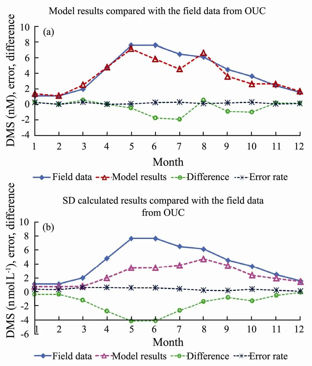
Fig.12 Monthly mean time series of DMS, and difference and error ratio comparisons (a), for the G93 model simulated DMS results with the field data; (b), for the calculated results using SD method and the field data.
The different calculation methods caused the error (Qu., 2020). The field data is also compared with the calculated results using SD method. The mean increased error rate of the model simulation result compared to the field data is 15.7%, the mean increased error rate of the calculated DMS compared to the field data of OUC is around 36.9%. The difference of simulated results and calculated results compared to the field data are clearly shown in Figs.12(a) and 12(b). Slightly bigger error occurred during May to July for model simulations and field data (Fig.12(a)), and even larger error occurred during May to June for SD method results comparing to the field data (Fig.12(b)). The peak of DMS is matched well in our simulated results. We conclude that our G93 model simu- lation results are closer to the field data comparing to those using SD method.
5 Conclusions
The distributions and correlations of CHL and AOD are studied for the time period (2011–2019) in the ECMS. CHL peaked from middle March to late April, apart from the late peak in May 2014 and in middle November 2017. There was no obvious trend in the timing of the peak during the study period. The phytoplankton bloom spread over the northern and middle regions as well as southwest region of the ECMS. CHL peaks appear along the coast of the study region during summer and winter months, although there was a second peak in October. Annual average of CHL decreased around 10% during the 9 year study period. However, AOD had no significant trend during this period. Positive correlations of about 0.5 between CHL and AOD were found in the study region, with higher correlations appeared along Jiangsu Province and Zhejiang Province coastal waters. This suggests a possible influence of DMS-derived aerosol in the local ECMS atmosphere. The positive correlation region is stronger in the southern region, and negative correlations in the northern region and offshore in the southern region.
DMS sensitivity analysis shows that the S:N ratio of phytoplankton is the most sensitive parameter for phytoplankton biomass growth. A genetic algorithm technique (Holland, 1975) is used to calibrate key parameters based on MODIS satellite CHL data and DMS field data obtained from OUC. Our simulated results show that our results are closer to the field data comparing to the calculated results from SD method. The elevated CHL concentration along the west coast would lead to increased sea- water concentrations of DMS (Yang., 2011; Zhang., 2014, 2017), and an increase in DMS sea-to-air fluxes along the coastal waters.
Acknowledgements
Great thanks should first go to the postgraduate student Zhiwei Xu, for his DMS model parameters calibrations. Special thanks should go to several undergraduate students from Nantong University Liyan Guo, Rui Wang, Yang Yang, Zheng Liu and Shan Yan, for calculating the regional mean profiles and distributions for CHL, AOD, CLD, SST and MLD. Thanks are to the MSc graduate Li Zhao, for her DMS calculated results using SD method. Further thanks should go to the Ocean University of China (OUC) for providing the field data of DMS concentrations in year 2015. Thanks are to Giovanni in Ear- thdata (the Bridge Between Data and Science in the NASA’s earth science data sets group) for providing a web-based tool, for better visualizations of CHL and AOD images. We acknowledge the Naval Research Laboratory Remote Sensing Division, the Naval Center for Space Technology, and the National Polar-orbiting Operational Environmental Satellite System (NPOESS) Integrated Program Office (IPO) for providing satellite-based WIND and SST data. Thanks are to NASA Goddard Earth Science (GES) and Information Services Center (DISC) team for providing cloud cover data. More thanks should go to Dr. David L. Carroll from CU Aerospace, for providing the genetic algorithm Fortran code.
Anderson, T. R., Spall, S. A., Yool, A., Cipollini, P., Challenor, P. G., and Fasham, M. J. R., 2001. Global fields of sea surface dimethylsulfide predicted from chlorophyll, nutrients and light., 30: 1-20.
Bates, T. S., Lamb, B. K., Guenther, A., Dignon, J., and Stoiber, R. E., 1992. Sulfur emissions to the atmosphere from natural sources., 14: 315-337.
Belviso, S., Bopp, L., Moulin, C., Orr, J. C., Anderson, T. R., Aumont, O.,., 2004. Comparison of global climatological maps of sea surface dimethyl sulfide., 18: 2-11.
Blomquist, B. W., Fairall, C. W., Huebert, B. J., Kieber, D. J., and Westby, G. R., 2006. DMS sea-air transfer velocity: Direct measurements by eddy covariance and parameterization based on the NOAA/COARE gas transfer model., 33: 17-23.
Chang, J., Shiah, F. K., Gong, G. C., and Chiang, K. P., 2003. Cross-shelf variation in carbon-to-chlorophyll a ratios in the East China Sea, summer 1998., 50: 1237-1247.
Charlson, R. J., Lovelock, J. E., Andreae, M. O., and Warren, S. G., 1987. Oceanic phytoplankton, atmospheric sulphur, cloud albedo and climate., 326: 655-661.
Chen, Y. L. L., Chen, H. Y., Gong, G. C., Lin, Y. H., Jan, S., and Takahashi, M., 2004. Phytoplankton production during a su- mmer coastal upwelling in the East China Sea., 24: 1321-1338.
Cropp, R. A., Norbury, J., Gabric, A. J., and Braddock, R. D., 2004. Modeling dimethylsulphide production in the upper ocean., 18: 43-49.
Doney, S. C., Glover, D. M., and Najjar, R. G., 1996. A new coupled, one-dimensional biological-physical model for the upper ocean: Applications to the JGOFS Bermuda Atlantic Time-series Study (BATS) site., 43: 591-624.
Erickson, D. J., Ghan, S. J., and Penner, J. E., 1990. Global ocean-to-atmosphere dimethyl sulfide flux., 95: 7543-7552.
Gabric, A. J., Gregg, W., Najjar, R., Erickson, D., and Matrai, P., 2001. Modelling the biogeochemical cycle of simethylsulfide in the upper ocean: A review., 126: 1-16.
Gabric, A. J., Matrai, P. A., and Vernet, M., 1999. Modelling the production and cycling of dimethylsulphide during the vernal bloom in the Barnents Sea., 51B: 919-937.
Gabric, A. J., Murray, N., Stone, L., and Kohl, M., 1993. Modelling the production of dimethylsulfide during a phytoplankton bloom., 98: 22805-22816.
Gabric, A. J., Qu, B., Matrai, P. A., and Hirst, A. C., 2005. The simulated response of dimethylsulfide production in the Arctic Ocean to global warming., 57: 391-403.
Galí, M., and Simó, R., 2015. A meta-analysis of oceanic DMS and DMSP cycling processes: Disentangling the summer paradox., 29: 496-515.
Holland, J. H., 1975.University of Michigan Press, Michigan, 1-24.
Huang, T. H., Chen, C. T. A., Lee, J., Wu, C. R., Wang, Y. L., Bai, Y.,., 2019. East China Sea increasingly gains limiting nutrient P from South China Sea., 9: 5648.
Jiang, Z., Chen, J., Zhou, F., Shou, L., Chen, Q., Tao, B.,., 2015. Controlling factors of summer phytoplankton community in the Changjiang (Yangtze River) Estuary and adjacent East China Sea shelf., 101: 71-84.
Jones, A., Roberts, D. L., Woodage, M. J., and Johnson, C. E., 2001. Indirect sulphate aerosol forcing in a climate model with an interactive sulphur cycle., 106: 20293-20310.
Kettle, A. J., and Andreae, M. O., 1999. A global database of sea surface dimethysulfide (DMS) meansurements and a procedure to predict sea surface DMS as a function of latitude, lon- gitude, and month., 13: 399- 444.
Kettle, A. J., and Andreae, M. O., 2000. Flux of dimethylsulfide from the ocean: A comparison of updated data sets and flux models., 105: 26793-26808.
Kim, T. W., Lee, K., Najjar, R., Jeong, H. D., and Jeong, H. J., 2011. Increasing N abundance in the northwestern Pacific Ocean due to atmospheric nitrogen deposition., 334: 505-509.
Kong, C. E., Yoo, S., and Jang, C. J., 2019. East China Sea ecosystem under multiple stressors: Heterogeneous responses in the sea surface chlorophyll-a., 151: 103078.
Liss, P. S., and Merlivat, L., 1986.Patrick, B. M., ed., Hingham, 113- 127.
Liu, X., Laws, E. A., Xie, Y., Wang, L., Lin, L., and Huang, B., 2019. Uncoupling of seasonal variations between phytoplan- kton chlorophylland production in the East China Sea., 124: 2400- 2415.
Liu, W. C., Wang, R., and Li, C. L., 1998. C/N Ratios of Particulate Organic Matter In The East China Sea.a, 29 (5): 467-470.
Mackey, K. R. M., Kavanaugh, M. T., Wang, F., Chen, Y., Liu, F., Glover, D. M.,., 2017. Atmospheric and fluvial nutrients fuel algal blooms in the East China Sea., 4: 10-18, DOI: 10.3389/fmars.2017.00002.
Masotti, I., Belviso, S., Alvain, S., Johnson, J. E., Bates, T. S., Tortell, P. D.,., 2010. Spatial and temporal variability of the dimethylsulfide to chlorophyll ratio in the surface ocean: An assessment based on phytoplankton group dominance determined from space., 7: 3215.
Nunes-Neto, N., Carmo, R., and El-Hani, C., 2011. The relationships between marine phytoplankton, dimethylsulphide and the global climate: The CLAW hypothesis as a Lakatosian progressive problemshift., 23: 169-186.
Qu, B., and Gabric, A. J., 2010. Using genetic algorithm to calibrate a dimethylsulfide production model in the Arctic Ocean., 28: 1-10.
Qu, B., and Liu, X., 2020. The effect of wind and temperature to phytoplankton biomass during blooming season in Barents Sea., 91: 101157.
Qu, B., Gabric, A. J., Zeng, M., and Lu, Z., 2016. Dimethylsulfide model calibration in the Barents Sea using a genetic algorithm and neural network., 13: 413-424.
Qu, B., Gabric, A. J., Zeng, M., Xi, J., Jiang, L., and Zhao, L., 2017. Dimethylsulfide model calibration and parametric sensitivity analysis for the Greenland Sea., 13: 13- 22.
Simó, R., 2004. From cells to globe: Approaching the dynamics of DMS(P) in the ocean at multiple scales., 61: 673-684.
Simó, R., and Dachs, J., 2002. Global ocean emission of dime- thylsulfide predicted from biogeophysical data., 16: 1078.
Stefels, J., Steinke, M., Turner, S., Malin, G., and Belviso, S., 2007. Environmental constraints on the production and removal of the climatically active gas dimethylsulphide (DMS) and implications for ecosystem modelling., 83: 245-275.
Tang, D., Di, B., Wei, G., Ni, I. H., Oh, I. S., and Wang, S., 2006. Spatial, seasonal and species variations of harmful algal blooms in the South Yellow Sea and East China Sea., 568: 245-253.
Wanninkhof, R., 1992. Relationship between wind speed and gas exchange over the ocean., 97: 7373-7382.
Xu, Z., Chen, Y., Meng, X., Wang, F., and Zheng, Z., 2016. Phytoplankton community diversity is influenced by environ- mental factors in the coastal East China Sea., 51: 107-118.
Yang, G. P., Zhang, H. H., Zhou, L. M., and Yang, J., 2011. Temporal and spatial variations of dimethylsulfide (DMS) and dimethylsulfoniopropionate (DMSP) in the East China Sea and the Yellow Sea., 31: 1325- 1335.
Zeng, X., He, R., and Zong, H., 2017. Variability of Changjiang diluted water revealed by a 45-year long-term ocean hindcast and self-organizing maps analysis., 146: 37-46.
Zhang, S. H., Sun, J., and Liu, J. E. A., 2017. Spatial distributions of dimethyl sulfur compounds, DMSP-lyase activity, and phytoplankton community in the East China Sea during fall., 133: 59-72.
Zhang, S.H., Yang, G.P., Zhang, H.H.,and Yang, J., 2014. Spatial variation of biogenic sulfur in the South Yellow Sea and the East China Sea during summer and its contribution to atmospheric sulfate aerosol., 488-489: 157-167.
March 4, 2021;
May 19, 2021;
May 27, 2021
© Ocean University of China, Science Press and Springer-Verlag GmbH Germany 2022
. E-mail: qubo@nte.edu.cn
(Edited by Ji Dechun)
猜你喜欢
中国南方果树(2022年4期)2022-08-03
农业工程学报(2022年6期)2022-06-27
保鲜与加工(2021年1期)2021-02-06
河北果树(2020年4期)2020-11-26
中国生殖健康(2019年12期)2019-01-07
山东农业科学(2016年11期)2016-12-17
江苏农业科学(2016年9期)2016-11-28
恋爱婚姻家庭·养生版(2016年9期)2016-09-07
热带农业工程(2014年1期)2014-08-19
 Journal of Ocean University of China2022年2期
- Journal of Ocean University of China的其它文章
- Study of the Wind Conditions in the South China Sea and Its Adjacent Sea Area
- A Spatiotemporal Interactive Processing Bias Correction Method for Operational Ocean Wave Forecasts
- Characteristics Analysis and Risk Assessment of Extreme Water Levels Based on 60-Year Observation Data in Xiamen, China
- Underwater Target Detection Based on Reinforcement Learning and Ant Colony Optimization
- Polar Sea Ice Identification and Classification Based on HY-2A/SCAT Data
- Thermo-Rheological Structure and Passive Continental Margin Rifting in the Qiongdongnan Basin,South China Sea, China